A Highly effective EDA Device: Group-By Aggregation

Discover ways to use group-by aggregation to uncover insights out of your knowledge

Exploratory Information Evaluation (EDA) is the core competency of an information analyst. Each day, knowledge analysts are tasked with seeing the “unseen,” or extracting helpful insights from an enormous ocean of knowledge.

On this regard, I’d like share a method that I discover useful for extracting related insights from knowledge: group-by aggregation.

To this finish, the remainder of this text will probably be organized as follows:

1. Clarification of group-by aggregation in Pandas
2. The dataset: Metro Interstate Visitors
3. Metro Visitors EDA

Group-By Aggregation

Group-by aggregation is an information manipulation approach that consists of two steps. First, we group the information primarily based on the values of particular columns. Second, we carry out some aggregation operations on prime of the grouped knowledge.

Group-by aggregation is very helpful when our knowledge is granular, as in typical reality tables (transactions knowledge) and time collection knowledge with slim intervals. By aggregating at the next degree than uncooked knowledge granularity, we are able to characterize the information in a extra compact manner — and should distill helpful insights within the course of.

In pandas, we are able to carry out group-by aggregation utilizing the next basic syntax kind.

df.groupby(['base_col']).agg(
  agg_col=('ori_col','agg_func')
)

The place base_col is the column whose values develop into the grouping foundation, agg_col is the brand new column outlined by taking agg_func aggregation on ori_col column.

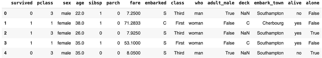
For instance, contemplate the notorious Titanic dataset whose 5 rows are displayed beneath.

import pandas as pd
import seaborn as sns

# import titanic dataset
titanic = sns.load_dataset("titanic")
titanic.head()

We will group this knowledge by the survived column after which mixture it by taking the median of the fare column to get the outcomes beneath.

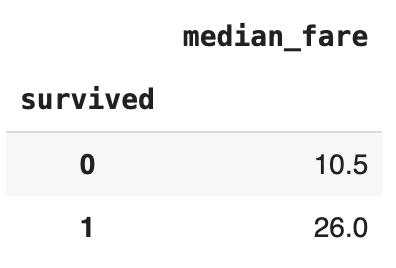
All of the sudden, we see an fascinating perception: survived passengers have the next fare median, which has greater than doubled. This might be associated to prioritizing security boats for greater cabin class passengers (i.e., passengers with greater fare tickets).

Hopefully, this easy instance demonstrates the potential of group by aggregation in gathering insights from knowledge. Okay then, let’s strive group-by-aggregation on a extra fascinating dataset!

The Dataset

We are going to use the Metro Interstate Visitors Quantity dataset. It’s a publicly obtainable dataset with a Inventive Frequent 4.0 license (which permits for sharing and adaptation of the dataset for any objective).

The dataset incorporates hourly Minneapolis-St Paul, MN visitors quantity for westbound I-94, which additionally consists of climate particulars from 2012–2018. The information dictionary info could be discovered on its UCI Machine Studying repo web page.

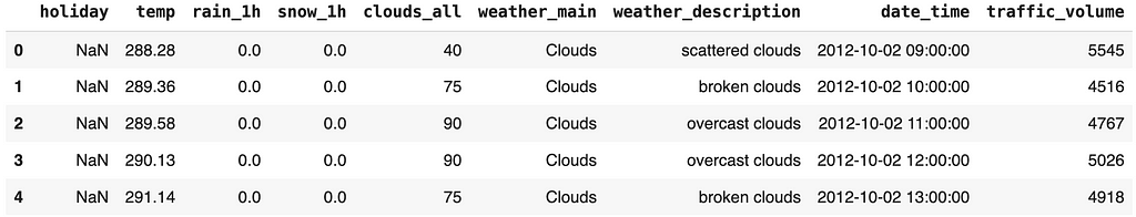
import pandas as pd

# load dataset
df = pd.read_csv("dir/to/Metro_Interstate_Traffic_Volume.csv")

# convert date_time column from object to correct datetime format
df['date_time'] = pd.to_datetime(df['date_time'])

# head
df.head()

For this weblog demo, we are going to solely use knowledge from 2016 onwards, as there’s lacking visitors knowledge from earlier intervals (attempt to test your self for train!).

Moreover, we are going to add a brand new column is_congested, which could have a worth of 1 if the traffic_volume exceeds 5000 and 0 in any other case.

# solely contemplate 2016 onwards knowledge
df = df.loc[df['date_time']>="2016-01-01",:]

# function engineering is_congested column
df['is_congested'] = df['traffic_volume'].apply(lambda x: 1 if x > 5000 else 0)

Metro Visitors EDA

Utilizing group-by aggregation as the principle weapon, we are going to attempt to reply the next evaluation questions.

1. How is the month-to-month development of the visitors quantity?
2. How is the visitors profile of every day in every week (Monday, Tuesday, and so on)?
3. How are typical hourly visitors quantity throughout 24 hours, damaged down by weekday vs weekend?
4. What are the highest climate situations that correspond to greater congestion charges?

Month-to-month development of visitors quantity

This query requires us to mixture (sum) visitors volumes at month degree. As a result of we don’t have the month column, we have to derive one primarily based on date_time column.

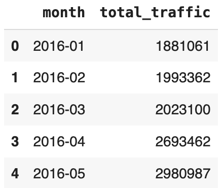
With monthcolumn in place, we are able to group primarily based on this column, and take the sum of traffic_volume. The codes are given beneath.

# create month column primarily based on date_time
# pattern values: 2016-01, 2026-02
df['month'] = df['date_time'].dt.to_period("M")

# get sum of traffic_volume by month
monthly_traffic = df.groupby('month', as_index=False).agg(
    total_traffic = ('traffic_volume', 'sum')
)

# convert month column to string for viz
monthly_traffic['month'] = monthly_traffic['month'].astype(str)

monthly_traffic.head()

We will draw line plot from this dataframe!

# draw time collection plot
plt.determine(figsize=(12,5))
sns.lineplot(knowledge=monthly_traffic, x ="month", y="total_traffic")
plt.xticks(rotation=90)
plt.title("Month-to-month Visitors Quantity")
plt.present()

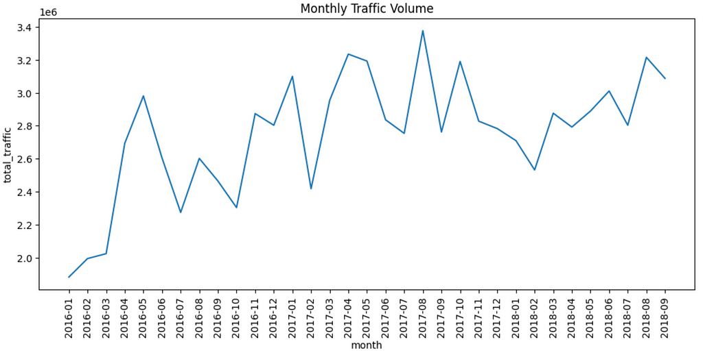
The above visualization exhibits that visitors quantity has typically elevated over the months inside the thought of knowledge interval.

Every day visitors profile

To research this, we have to create two extra columns: date and dayname. The previous is used as the first group-by foundation, whereas the latter is used as a breakdown when displaying the knowledge.

Within the following codes, we outline date and dayname columns. Afterward, we group-by primarily based on each columns to get the sum of traffic_volume. Be aware that since dayname is extra coarse (greater aggregation degree) than date , it successfully means we mixture primarily based on date values.

# create column date from date_time
# pattern values: 2016-01-01, 2016-01-02
df['date'] = df['date_time'].dt.to_period('D')

# create  dayname column
# pattern values: Monday, Tuesday
df['dayname'] = df['date_time'].dt.day_name()

# get sum of visitors, at date degree
daily_traffic = df.groupby(['dayname','date'], as_index=False).agg(
    total_traffic = ('traffic_volume', 'sum')
)

# map dayname to quantity for viz later
dayname_map = {
    'Monday': 1,
    'Tuesday': 2,
    'Wednesday': 3,
    'Thursday': 4,
    'Friday': 5,
    'Saturday': 6,
    'Sunday': 7
}

daily_traffic['dayname_index'] = daily_traffic['dayname'].map(dayname_map)
daily_traffic = daily_traffic.sort_values(by='dayname_index')

daily_traffic.head()

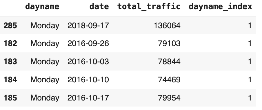
The above desk incorporates completely different realizations of day by day complete visitors quantity per day title. Field plot visualizations are acceptable to point out these variations of visitors quantity, permitting us to understand how visitors volumes differ on Monday, Tuesday, and so on.

# draw boxplot per day title
plt.determine(figsize=(12,5))
sns.boxplot(knowledge=daily_traffic, x="dayname", y="total_traffic")
plt.xticks(rotation=90)
plt.title("Every day Visitors Quantity")
plt.present()

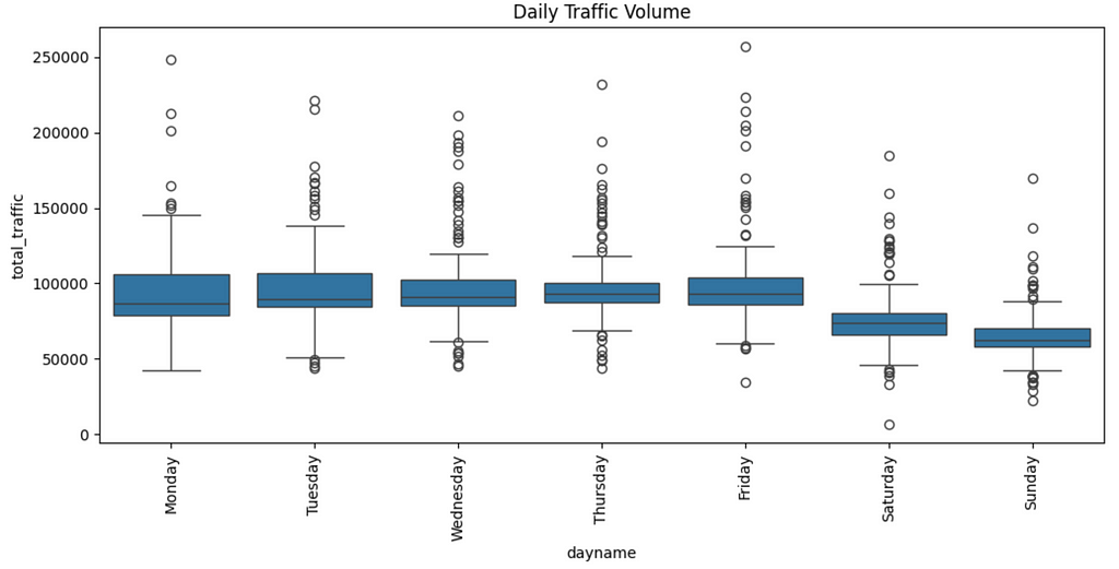
The above plot exhibits that every one weekdays (Mon-Fri) have roughly the identical visitors density. Weekends (Saturday and Sunday) have decrease visitors, with Sunday having the least of the two.

Hourly visitors patterns, damaged down by weekend standing

Comparable as earlier questions, we have to engineer two new columns to reply this query, i.e., hour and is_weekend.

Utilizing the identical trick, we are going to group by is_weekend and hour columns to get averages of traffic_volume.

# extract hour digit from date_time
# pattern values: 1,2,3
df['hour'] = df['date_time'].dt.hour

# create is_weekend flag primarily based on dayname
df['is_weekend'] = df['dayname'].apply(lambda x: 1 if x in ['Saturday', 'Sunday'] else 0)

# get common visitors at hour degree, damaged down by is_weekend flag
hourly_traffic = df.groupby(['is_weekend','hour'], as_index=False).agg(
    avg_traffic = ('traffic_volume', 'imply')
)

hourly_traffic.head()

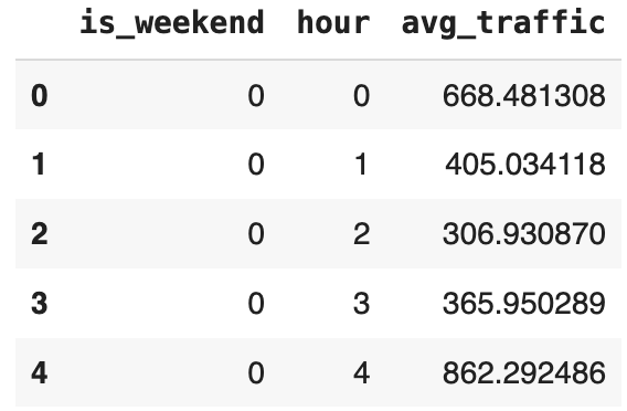
For the visualization, we are able to use bar chart with break down on is_weekend flag.

# draw as barplot with hue = is_weekend
plt.determine(figsize=(20,6))
sns.barplot(knowledge=hourly_traffic, x='hour', y='avg_traffic', hue='is_weekend')
plt.title("Common Hourly Visitors Quantity: Weekdays (blue) vs Weekend (orange)", fontsize=14)
plt.present()

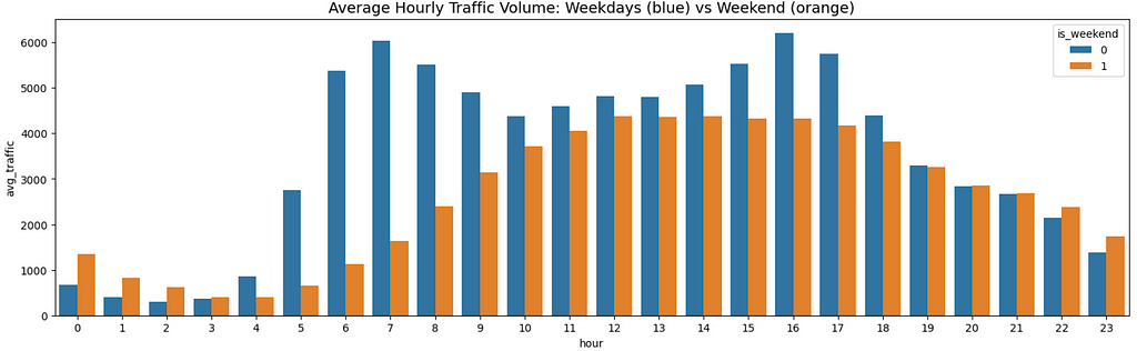
Very fascinating and wealthy visualization! Observations:

1. Weekday visitors has a bimodal distribution sample. It reaches its highest visitors between 6 and eight a.m. and 16 and 17 p.m. That is considerably intuitive as a result of these time home windows characterize individuals going to work and returning dwelling from work.
2. Weekend visitors follows a very completely different sample. It has a unimodal form with a big peak window (12–17). Regardless of being typically inferior (much less visitors) to weekday equal hours, it’s value noting that weekend visitors is definitely greater throughout late-night hours (22–2). This might be as a result of individuals are staying out till late on weekend nights.

Prime climate related to congestion

To reply this query, we have to calculate congestion price for every climate situation within the dataset (using is_congested column). Can we calculate it utilizing group-by aggregation? Sure we can!

The important thing commentary to make is that the is_congested column is binary. Thus, the congestion price could be calculated by merely averaging this column! Common of a binary column equals to sum(worth 1)/depend(all rows) — let that sink in for a second if it’s new for you.

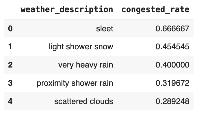
Based mostly on this neat commentary, all we have to do is take the common (imply) of is_congested grouped by weather_description. Following that, we kind the outcomes descending by congested_rate.

# price of congestion (is_congested) , grouped by climate description
congested_weather = df.groupby('weather_description', as_index=False).agg(
    congested_rate = ('is_congested', 'imply')
).sort_values(by='congested_rate', ascending=False, ignore_index=True)

congested_weather.head()

# draw as barplot
plt.determine(figsize=(20,6))
sns.barplot(knowledge=congested_weather, x='weather_description', y='congested_rate')
plt.xticks(rotation=90)
plt.title('Prime Climate with Excessive Congestion Charges')
plt.present()

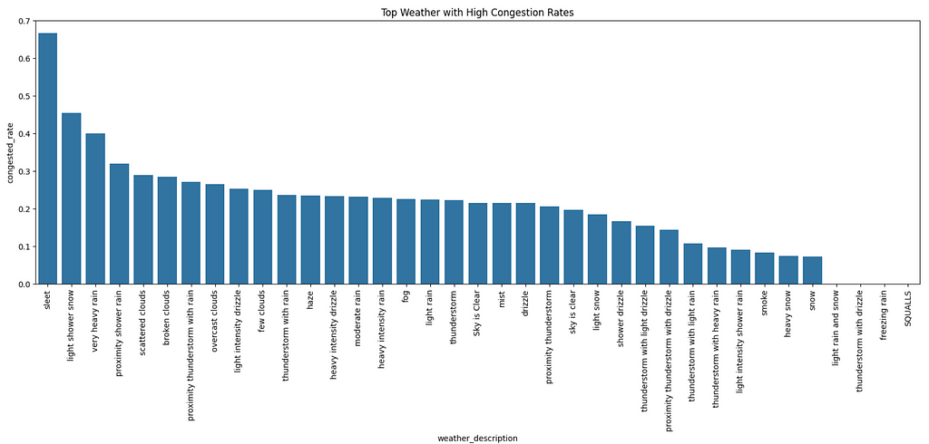
From the graph:

1. The highest three climate situations with the very best congestion charges are sleet, mild bathe snow, and really heavy rain.
2. In the meantime, mild rain and snow, thunderstorms with drizzle, freezing rain, and squalls haven’t brought about any congestion. Folks have to be staying indoors throughout such excessive climate!

Closing

On this weblog put up, we coated tips on how to use group-by-aggregation in EDA workout routines. As we are able to see, this system is extremely efficient in revealing fascinating, helpful insights from knowledge, significantly when coping with granular knowledge.

I hope you may observe doing group-by aggregation throughout your subsequent EDA mission! All in all, thanks for studying, and let’s join with me on LinkedIn! 👋

---

A Highly effective EDA Device: Group-By Aggregation was initially printed in In direction of Information Science on Medium, the place individuals are persevering with the dialog by highlighting and responding to this story.

Supply hyperlink