


 for Gaming&Video Enhancing (16GB RAM)")


, SSD (1TB NVME), RAM (16gbgb), with Tempered Glass Aspect Panel On Gaming Cupboard")


Not All HNSW Indices Are Made Equally
Overcoming Main HNSW Challenges to Enhance the Effectivity of Your AI Manufacturing Workload
The Hierarchical Navigable Small World (HNSW) algorithm is thought for its effectivity and accuracy in high-scale knowledge searches, making it a preferred selection for search duties and AI/LLM functions like RAG. Nevertheless, establishing and sustaining an HNSW index comes with its personal set of challenges. Let’s discover these challenges, supply some methods to beat them, and even see how we will kill two birds with one stone by addressing simply one among them.
Reminiscence Consumption
As a consequence of its hierarchical construction of embeddings, one of many main challenges of HNSW is its excessive reminiscence utilization. However not many notice that the reminiscence situation extends past the reminiscence required to retailer the preliminary index. It’s because, as an HNSW index is modified, the reminiscence required to retailer nodes and their connections will increase much more. This shall be defined in better depth in a later part. Reminiscence consciousness is essential for the reason that extra reminiscence you want on your knowledge, the longer it should take to compute (search) over it, and the dearer it should get to keep up your workload.
Construct Time

Within the course of of making an index, nodes are added to the graph based on how shut they’re to different nodes on the graph. For each node, a dynamic checklist of its closest neighbors is stored at every degree of the graph. This course of includes iterating over the checklist and performing similarity searches to find out if a node’s neighbors are nearer to the question. This computationally heavy iterative course of considerably will increase the general construct time of the index, negatively impacting your customers’ expertise and costing you extra in cloud utilization bills.
Parameter Tuning
HNSW requires predefined configuration parameters in it’s construct course of. Optimizing HNSW these parameters: M (the variety of connections per node), and ef_construction (the scale of the dynamic checklist for the closest neighbors which is used throughout the index development) is essential for balancing search pace, accuracy and using reminiscence. Incorrect parameter settings can result in poor efficiency and elevated manufacturing prices. Effective-tuning these parameters is exclusive for each index and is a steady course of that requires usually re-building of indices.
Rebuilding Indices

Rebuilding an HNSW index is among the most resource-intensive facets of utilizing HNSW in manufacturing workloads. In contrast to conventional databases, the place knowledge deletions will be dealt with by merely deleting a row in a desk, utilizing HNSW in a vector database usually requires a whole rebuild to keep up optimum efficiency and accuracy.
Why is Rebuilding Mandatory?
Due to its layered graph construction, HNSW shouldn’t be inherently designed for dynamic datasets that change continuously. Including new knowledge or deleting current knowledge is important for sustaining up to date knowledge, particularly to be used circumstances like RAG, which goals to enhance search relevence.
Most databases work on an idea known as “exhausting” and “mushy” deletes. Exhausting deletes completely take away knowledge, whereas mushy deletes flag knowledge as ‘to-be-deleted’ and take away it later. The difficulty with mushy deletes is that the to-be-deleted knowledge nonetheless makes use of vital reminiscence till it’s completely eliminated. That is notably problematic in vector databases that use HNSW, the place reminiscence consumption is already a major situation.
HNSW creates a graph the place nodes (vectors) are related primarily based on their proximity within the vector area, and traversing on an HNSW graph is finished like a skip-list. With the intention to help that, the layers of the graph are designed in order that some layers have only a few nodes. When vectors are deleted, particularly these on layers which have only a few nodes that function important connectors within the graph, the entire HNSW construction can change into fragmented. This fragmentation could result in nodes (or layers) which are disconnected from the principle graph, which require rebuilding of your entire graph, or on the very least will lead to a degradation within the effectivity of searches.
HNSW then makes use of a soft-delete method, which marks vectors for deletion however doesn’t instantly take away them. This strategy lowers the expense of frequent full rebuilds, though periodic reconstruction remains to be wanted to keep up the graph’s optimum state.
Addressing HNSW Challenges
So what methods do we have now to handle these challenges? Listed below are a couple of that labored for me:
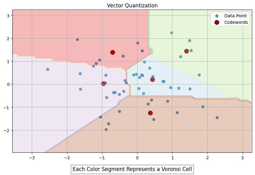
- Vector Quantization — Vector quantization (VQ) is a course of that maps k-dimensional vectors from a vector area ℝ^ok right into a finite set of vectors often known as codewords (for instance, by utilizing the Linde-Buzo-Grey (LBG) algorithm), which type a codebook. Every codeword Yi has an related area known as a Voronoi area, which partitions your entire area ℝ^ok into areas primarily based on proximity to the codewords (see graph beneath). When an enter vector is supplied, it’s in contrast with every codeword within the codebook to seek out the closest match. That is performed by figuring out the codeword within the codebook with the minimal Euclidean distance to the enter vector. As a substitute of transmitting or storing your entire enter vector, the index of the closest codeword is distributed (encoding). When retrieving the vector (decoding), the decoder retrieves the corresponding codeword from the codebook. The codeword is used as an approximation of the unique enter vector. The reconstructed vector is an approximation of the unique knowledge, nevertheless it sometimes retains probably the most vital traits as a result of nature of the VQ course of. VQ is one well-liked option to scale back index construct time and the quantity of reminiscence used to retailer the HNSW graph. Nevertheless, it is very important perceive that it’ll additionally scale back the accuracy of your search outcomes.
2. Frequent index rebuilds — One option to overcome the HNSW increasing reminiscence problem is to continuously rebuild your index so that you just do away with nodes which are marked as “to-be-deleted”, which take up area and scale back search pace. Think about making a duplicate of your index throughout these instances so that you don’t endure full downtime (Nevertheless, this may require quite a lot of reminiscence — an already large situation with HNSW).
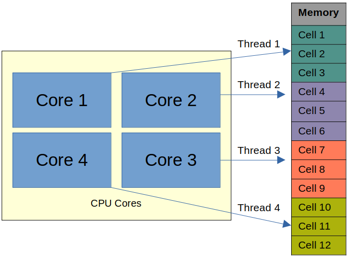
3. Parallel Index Construct — Constructing an index in parallel includes partitioning the info and the allotted reminiscence and distributing the indexing course of throughout a number of CPU cores. On this course of, all operations are mapped to obtainable RAM. As an example, a system would possibly partition the info into manageable chunks, assign every chunk to a distinct processor core, and have them construct their respective elements of the index concurrently. This parallelization permits for higher utilization of the system’s assets, leading to sooner index creation instances, particularly for big datasets. This can be a sooner option to construct indices in comparison with conventional single-threaded builds; nonetheless, challenges come up when your entire index can’t match into reminiscence or when a CPU doesn’t have sufficient cores to help your workload within the required timeframe.
Utilizing Customized Construct Accelerators: A Totally different Strategy
Whereas the above methods can assist, they usually require vital experience and growth. Introducing GXL, a brand new paid-for instrument designed to reinforce HNSW index development. It makes use of the APU, GSI Know-how’s compute-in-memory Associative Processing Unit, which makes use of its tens of millions of bit processors to carry out computation throughout the reminiscence. This structure allows large parallel processing of nearest neighbor distance calculations, considerably accelerating index construct instances for large-scale dynamic datasets. It makes use of a customized algorithm that mixes vector quantization and overcomes the similarity search bottleneck with parallalism utilizing distinctive {hardware} to scale back the general index construct time.
Let’s try some benchmark numbers:
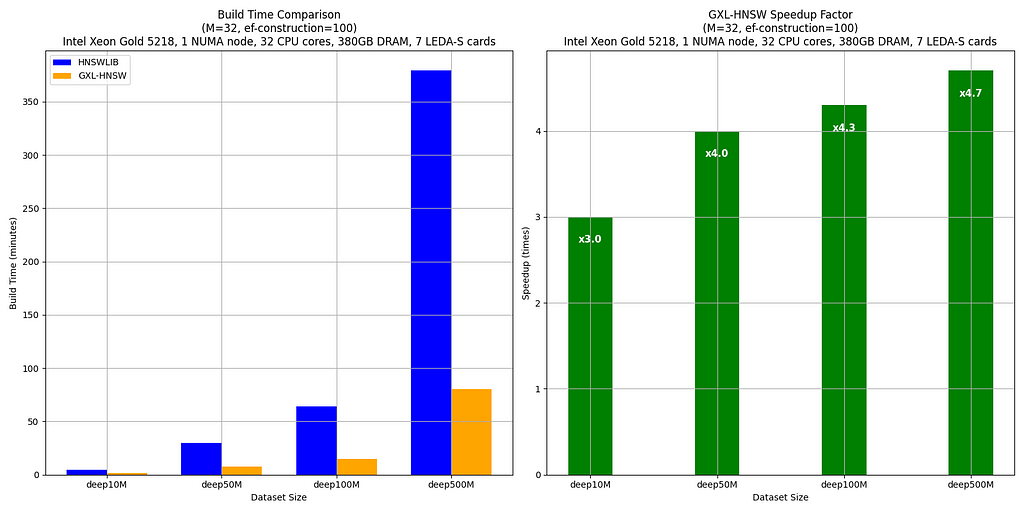
The benchmarks examine the construct instances of HNSWLIB and GXL-HNSW for numerous dataset sizes (deep10M, deep50M, deep100M, and deep500M — all subsets of deep1B) utilizing the parameters M = 32 and ef-construction = 100. These assessments have been performed on a server with an Intel(R) Xeon(R) Gold 5218 CPU @ 2.30GHz, utilizing one NUMA node (32 CPU cores, 380GB DRAM, and seven LEDA-S APU playing cards).
The outcomes clearly present that GXL-HNSW considerably outperforms HNSWLIB throughout all dataset sizes. As an example, GXL-HNSW builds the deep10M dataset in 1 minute and 35 seconds, whereas HNSWLIB takes 4 minutes and 44 seconds, demonstrating a speedup issue of three.0. Because the dataset dimension will increase, the effectivity of GXL-HNSW turns into even better, with speedup components of 4.0 for deep50M, 4.3 for deep100M, and 4.7 for deep500M. This constant enchancment highlights GXL-HNSW’s higher efficiency in dealing with large-scale knowledge, making it a extra environment friendly selection for large-scale dataset similarity searches.
In conclusion, whereas HNSW is very efficient for vector search and AI pipelines, it faces robust challenges corresponding to sluggish index constructing instances and excessive reminiscence utilization, which turns into even better due to HNSW’s complicated deletion administration. Methods to handle these challenges embrace optimizing your reminiscence utilization by frequent index rebuilding, implementing vector quantization to your index, and parallelizing your index development. GXL gives an strategy that successfully combines a few of these methods. These strategies assist preserve accuracy and effectivity in methods counting on HNSW. By decreasing the time it takes to construct indices, index rebuilding isn’t as a lot of a time-intensive situation because it as soon as was, enableing us to kill two birds with one stone — fixing each the reminiscence growth downside and lengthy index constructing instances. Take a look at out which methodology fits you greatest, and I hope this helps enhance your general manufacturing workload efficiency.
Not All HNSW Indices Are Made Equaly was initially printed in In direction of Information Science on Medium, the place individuals are persevering with the dialog by highlighting and responding to this story.