


-Powered by MediaTek Dimensity 6080 Processor|120Hz FHD+ Show|50MP+8MP Ultrawide Digicam|16MP FrontCamera|33W Quick Charging|Upto 16GB ExpandableRAM")

 | World’s 1st 4nm Dimensity 9000 5G Processor | Curved AMOLED Show | 64MP RGBW Digicam | 5GB Reminiscence Fusion | 50% cost in simply 20 minutes")

")


Solid a versatile internet that solely retains large fish
Notice: The code used on this article makes use of three customized scripts, data_cleaning, data_review, and , eda, that may be accessed by a public GitHub repository.

It is sort of a stretchable fishing internet that retains ‘all the massive fish’ Zou & Hastie (2005) p. 302
Background
Linear regression is a generally used educating software in information science and, underneath the suitable situations (e.g., linear relationship between the unbiased and dependent variables, absence of multicollinearity), it may be an efficient methodology for predicting a response. Nevertheless, in some situations (e.g., when the mannequin’s construction turns into complicated), its use might be problematic.
To handle among the algorithm’s limitations, penalization or regularization methods have been recommended [1]. Two in style strategies of regularization are ridge and lasso regression, however selecting between these strategies might be troublesome for these new to the sphere of information science.
One strategy to picking between ridge and lasso regression is to look at the relevancy of the options to the response variable [2]. When nearly all of options within the mannequin are related (i.e., contribute to the predictive energy of the mannequin), the ridge regression penalty (or L2 penalty) ought to be added to linear regression.
When the ridge regression penalty is added, the associated fee perform of the mannequin is:
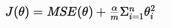
- θ = the vector of parameters or coefficients of the mannequin
- α = the general energy of the regularization
- m = the variety of coaching examples
- n = the variety of options within the dataset
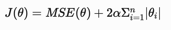
When nearly all of options are irrelevant (i.e., don’t contribute to the predictive energy of the mannequin), the lasso regression penalty (or L1 penalty) ought to be added to linear regression.
When the lasso regression penalty is added, the associated fee perform of the mannequin is:
Relevancy might be decided by guide evaluate or cross validation; nonetheless, when working with a number of options, the method turns into time consuming and computationally costly.
An environment friendly and versatile answer to this problem is utilizing elastic internet regression, which mixes the ridge and lasso penalties.
The fee perform for elastic internet regression is:
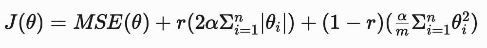
- r = the blending ratio between ridge and lasso regression.
When r is 1, solely the lasso penalty is used and when r is 0 , solely the ridge penalty is used. When r is a worth between 0 and 1, a combination of the penalties is used.
Along with being well-suited for datasets with a number of options, elastic internet regression has different attributes that make it an interesting software for information scientists [1]:
- Automated choice of related options, which ends up in parsimonious fashions which are simple to interpret
- Steady shrinkage, which regularly reduces the coefficients of much less related options in the direction of zero (against an instantaneous discount to zero)
- Capacity to pick teams of correlated options, as an alternative of choosing one function from the group arbitrarily
As a consequence of its utility and suppleness, Zou and Hastie (2005) in contrast the mannequin to a “…stretchable fishing internet that retains all the massive fish.” (p. 302), the place large fish are analogous to related options.
Now that now we have some background, we are able to transfer ahead to implementing elastic internet regression on an actual dataset.
Implementation
An incredible useful resource for information is the College of California at Irvine’s Machine Studying Repository (UCI ML Repo). For the tutorial, we’ll use the Wine High quality Dataset [3], which is licensed underneath a Inventive Commons Attribution 4.0 Worldwide license.
The perform displayed under can be utilized to acquire datasets and variable info from the UCI ML Repo by getting into the identification quantity because the parameter of the perform.
pip set up ucimlrepo # except already put in
from ucimlrepo import fetch_ucirepo
import pandas as pd

def fetch_uci_data(id):
    """
    Perform to return options datasets from the UCI ML Repository.

    Parameters
    ----------
    id: int
        Figuring out quantity for the dataset

    Returns
    ----------
    df: df
        Dataframe with options and response variable
    """
    dataset = fetch_ucirepo(id=id)

    options = pd.DataFrame(dataset.information.options)
    response = pd.DataFrame(dataset.information.targets)
    df = pd.concat([features, response], axis=1)

    # Print variable info
    print('Variable Data')
    print('--------------------')
    print(dataset.variables)

    return(df)
# Wine High quality's identification quantity is 186
df = fetch_uci_data(186)
A pandas dataframe has been assigned to the variable “df” and details about the dataset has been printed.
Exploratory Knowledge Evaluation
Variable Data
--------------------
                    identify     position         kind demographic
0          fixed_acidity  Function   Steady        None
1       volatile_acidity  Function   Steady        None
2            citric_acid  Function   Steady        None
3         residual_sugar  Function   Steady        None
4              chlorides  Function   Steady        None
5    free_sulfur_dioxide  Function   Steady        None
6   total_sulfur_dioxide  Function   Steady        None
7                density  Function   Steady        None
8                     pH  Function   Steady        None
9              sulphates  Function   Steady        None
10               alcohol  Function   Steady        None
11               high quality   Goal      Integer        None
12                 shade    Different  Categorical        None

               description models missing_values
0                     None  None             no
1                     None  None             no
2                     None  None             no
3                     None  None             no
4                     None  None             no
5                     None  None             no
6                     None  None             no
7                     None  None             no
8                     None  None             no
9                     None  None             no
10                    None  None             no
11  rating between 0 and 10  None             no
12            purple or white  None             no
Based mostly on the variable info, we are able to see that there are 11 “options”, 1 “goal”, and 1 “different” variables within the dataset. That is fascinating info — if we had extracted the info with out the variable info, we could not have identified that there have been information out there on the household (or shade) of wine. Presently, we gained’t be incorporating the “shade” variable into the mannequin, but it surely’s good to realize it’s there for future iterations of the venture.
The “description” column within the variable info means that the “high quality” variable is categorical. The information are doubtless ordinal, which means they’ve a hierarchical construction however the intervals between the info are usually not assured to be equal or identified. In sensible phrases, it means a wine rated as 4 just isn’t twice nearly as good as a wine rated as 2. To handle this problem, we’ll convert the info to the right data-type.
df['quality'] = df['quality'].astype('class')
To achieve a greater understanding of the info, we are able to use the countplot() methodology from the seaborn bundle to visualise the distribution of the “high quality” variable.
import seaborn as sns
import matplotlib.pyplot as plt

sns.set_theme(model='whitegrid') # optionally available

sns.countplot(information=df, x='high quality')
plt.title('Distribution of Wine High quality')
plt.xlabel('High quality')
plt.ylabel('Depend')
plt.present()
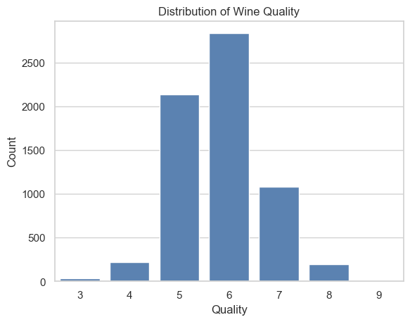
When conducting an exploratory information evaluation, creating histograms for numeric options is helpful. Moreover, grouping the variables by a categorical variable can present new insights. The best choice for grouping the info is “high quality”. Nevertheless, given there are 7 teams of high quality, the plots may turn out to be troublesome to learn. To simplify grouping, we are able to create a brand new function, “ranking”, that organizes the info on “high quality” into three classes: low, medium, and excessive.
def categorize_quality(worth):
 if 0 <= worth <= 3:
    return 0 # low ranking
 elif 4 <= worth <= 6:
    return 1 # medium ranking
 else:
    return # excessive ranking

# Create new column for 'ranking' information
df['rating'] = df['quality'].apply(categorize_quality)
To find out what number of wines are every group, we are able to use the next code:
df['rating'].value_counts()
ranking
1    5190
2    1277
0      30
Title: depend, dtype: int64
Based mostly on the output of the code, we are able to see that almost all of wines are categorized as “medium”.
Now, we are able to plot histograms of the numeric options teams by “ranking”. To plot the histogram we’ll want to make use of the gen_histograms_by_category() methodology from the eda script within the GitHub repository shared initially of the article.
import eda

eda.gen_histograms_by_category(df, 'ranking')
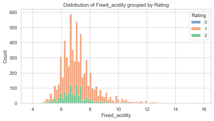
Above is among the plots generated by the strategy. A evaluate of the plot signifies there’s some skew within the information. To achieve a extra exact measure of skew, together with different statistics, we are able to use the get_statistics() methodology from the data_review script.
from data_review import get_statistics

get_statistics(df)
-------------------------
Descriptive Statistics
-------------------------
          fixed_acidity  volatile_acidity  citric_acid  residual_sugar    chlorides  free_sulfur_dioxide  total_sulfur_dioxide      density           pH    sulphates      alcohol      high quality
depend       6497.000000       6497.000000  6497.000000     6497.000000  6497.000000          6497.000000           6497.000000  6497.000000  6497.000000  6497.000000  6497.000000  6497.000000
imply           7.215307          0.339666     0.318633        5.443235     0.056034            30.525319            115.744574     0.994697     3.218501     0.531268    10.491801     5.818378
std            1.296434          0.164636     0.145318        4.757804     0.035034            17.749400             56.521855     0.002999     0.160787     0.148806     1.192712     0.873255
min            3.800000          0.080000     0.000000        0.600000     0.009000             1.000000              6.000000     0.987110     2.720000     0.220000     8.000000     3.000000
25%            6.400000          0.230000     0.250000        1.800000     0.038000            17.000000             77.000000     0.992340     3.110000     0.430000     9.500000     5.000000
50%            7.000000          0.290000     0.310000        3.000000     0.047000            29.000000            118.000000     0.994890     3.210000     0.510000    10.300000     6.000000
75%            7.700000          0.400000     0.390000        8.100000     0.065000            41.000000            156.000000     0.996990     3.320000     0.600000    11.300000     6.000000
max           15.900000          1.580000     1.660000       65.800000     0.611000           289.000000            440.000000     1.038980     4.010000     2.000000    14.900000     9.000000
skew           1.723290          1.495097     0.471731        1.435404     5.399828             1.220066             -0.001177     0.503602     0.386839     1.797270     0.565718     0.189623
kurtosis       5.061161          2.825372     2.397239        4.359272    50.898051             7.906238             -0.371664     6.606067     0.367657     8.653699    -0.531687     0.23232
In keeping with the histogram, the function labeled “fixed_acidity” has a skewness of 1.72 indicating vital right-skewness.
To find out if there are correlations between the variables, we are able to use one other perform from the eda script.
eda.gen_corr_matrix_hmap(df)
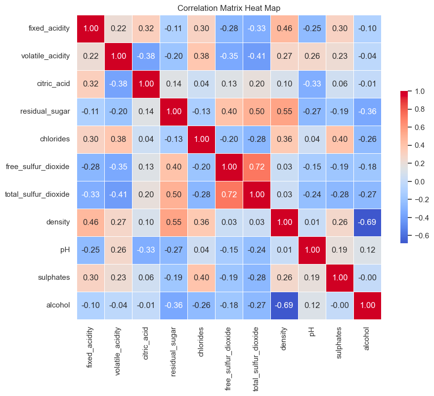
Though there a number of average and powerful relationships between options, elastic internet regression performs properly with correlated variables, subsequently, no motion is required [2].
Knowledge Cleansing
For the elastic internet regression algorithm to run accurately, the numeric information have to be scaled and the explicit variables have to be encoded.
To wash the info, we’ll take the next steps:
- Scale the info utilizing the the scale_data() methodology from the the data_cleaning script
- Encode the “high quality” and “ranking” variables utilizing the the get_dummies() methodology from pandas
- Separate the options (i.e., X) and response variable (i.e., y) utilizing the separate_data() methodology
- Break up the info into prepare and take a look at units utilizing train_test_split()
from sklearn.model_selection import train_test_split
from data_cleaning import scale_data, separate_data

df_scaled = scale_data(df)
df_encoded = pd.get_dummies(df_scaled, columns=['quality', 'rating'])

# Separate options and response variable (i.e., 'alcohol')
X, y = separate_data(df_encoded, 'alcohol')

# Create take a look at and prepare units
X_train, X_test, y_train, y_test = train_test_split(X, y, test_size =0.2, random_state=0)
Mannequin Constructing and Analysis
To coach the mannequin, we’ll use ElasticNetCV() which has two parameters, alpha and l1_ratio, and built-in cross validation. The alpha parameter determines the energy of the regularization utilized to the mannequin and l1_ratio determines the combo of the lasso and ridge penalty (it’s equal to the variable r that was reviewed within the Background part).
- When l1_ratio is ready to a worth of 0, the ridge regression penalty is used.
- When l1_ratio is ready to a worth of 1, the lasso regression penalty is used.
- When l1_ratio is ready to a worth between 0 and 1, a combination of each penalties are used.
Selecting values for alpha and l1_ratio might be difficult; nonetheless, the duty is made simpler by the usage of cross validation, which is constructed into ElasticNetCV(). To make the method simpler, you don’t have to supply an inventory of values from alpha and l1_ratio — you may let the strategy do the heavy lifting.
from sklearn.linear_model import ElasticNet, ElasticNetCV

# Construct the mannequin
elastic_net_cv = ElasticNetCV(cv=5, random_state=1)

# Practice the mannequin
elastic_net_cv.match(X_train, y_train)

print(f'Greatest Alpha: {elastic_net_cv.alpha_}')
print(f'Greatest L1 Ratio:{elastic_net_cv.l1_ratio_}')
Greatest Alpha: 0.0013637974514517563
Greatest L1 Ratio:0.5
Based mostly on the printout, we are able to see the most effective values for alpha and l1_ratio are 0.001 and 0.5, respectively.
To find out how properly the mannequin carried out, we are able to calculate the Imply Squared Error and the R-squared rating of the mannequin.
from sklearn.metrics import mean_squared_error

# Predict values from the take a look at dataset
elastic_net_pred = elastic_net_cv.predict(X_test)

mse = mean_squared_error(y_test, elastic_net_pred)
r_squared = elastic_net_cv.rating(X_test, y_test)

print(f'Imply Squared Error: {mse}')
print(f'R-squared worth: {r_squared}')
Imply Squared Error: 0.2999434011721803
R-squared worth: 0.7142939720612289
Conclusion
Based mostly on the analysis metrics, the mannequin performs reasonably properly. Nevertheless, its efficiency might be enhanced by some extra steps, like detecting and eradicating outliers, extra function engineering, and offering a particular set of values for alpha and l1_ratio in ElasticNetCV(). Sadly, these steps are past the scope of this easy tutorial; nonetheless, they could present some concepts for the way this venture might be improved by others.
Thanks for taking the time to learn this text. If in case you have any questions or suggestions, please depart a remark.
References
[1] H. Zou & T. Hastie, Regularization and Variable Choice By way of the Elastic Web, Journal of the Royal Statistical Society Sequence B: Statistical Methodology, Quantity 67, Situation 2, April 2005, Pages 301–320, https://doi.org/10.1111/j.1467-9868.2005.00503.x
[2] A. Géron, Palms-On Machine Studying with Scikit-Be taught, Keras & Tensorflow: Ideas, Instruments, and Methods to Construct Clever Methods (2021), O’Reilly.
[3] P. Cortez, A. Cerdeira, F. Almeida, T. Matos, & Reis,J.. (2009). Wine High quality. UCI Machine Studying Repository. https://doi.org/10.24432/C56S3T.
The way to Use Elastic Web Regression was initially revealed in In direction of Knowledge Science on Medium, the place individuals are persevering with the dialog by highlighting and responding to this story.