[ad_1]
Decoding the Math behind Q-Studying, Motion-Worth Capabilities, and Bellman Equations, and constructing them from scratch in Python.

Within the earlier article, we dipped our toes into the world of reinforcement studying (RL), protecting the fundamentals like how brokers study from their environment, specializing in a easy setup known as GridWorld. We went over the necessities — actions, states, rewards, and the right way to get round on this setting. If you happen to’re new to this or want a fast recap, it may be a good suggestion to take a look at that piece once more to get a agency grip on the fundamentals earlier than diving in deeper.
Reinforcement Studying 101: Constructing a RL Agent
At the moment, we’re able to take it up a bit. We are going to discover extra advanced points of RL, shifting from easy setups to dynamic, ever-changing environments and extra subtle methods for our brokers to navigate via them. We’ll dive into the idea of the Markov Resolution Course of, which is essential for understanding how RL works at a deeper degree. Plus, we’ll take a better take a look at Q-learning, a key algorithm in RL that reveals how brokers can study to make good selections in locations like GridWorld, even when issues are always altering.
Index
· 1: Past the Fundamentals
∘ 1.1: Dynamic Environments
· 2: Markov Resolution Course of
∘ 2.1: Understanding MDP
∘ 2.2: The Math Behind MDP
∘ 2.3: The Math Behind Bellman Equations
· 3: Deep Dive into Q-Studying
∘ 3.1: Fundamentals of Q-Studying
∘ 3.2: The Math Behind Q-Studying
· 4: Q-Studying From Scratch
∘ 4.1: The GridWorld Atmosphere
∘ 4.2: The Q-Studying Class
· 5: Subsequent Steps and Future Instructions
∘ 5.1: Present Issues and Limitations
∘ 5.2: Subsequent Steps
1: Past the Fundamentals
1.1: Dynamic Environments
After we first began exploring reinforcement studying (RL), we checked out easy, unchanging worlds. However as we transfer to dynamic environments, issues get much more fascinating. Not like static setups the place every little thing stays the identical, dynamic environments are all about change. Obstacles transfer, objectives shift, and rewards range, making these settings a lot nearer to the actual world’s unpredictability.
What Makes Dynamic Environments Particular?
Dynamic environments are key for instructing brokers to adapt as a result of they mimic the fixed modifications we face day by day. Right here, brokers have to do extra than simply discover the quickest path to a objective; they’ve to regulate their methods as obstacles transfer, objectives relocate, and rewards improve or lower. This steady studying and adapting are what may result in true synthetic intelligence.
Shifting again to the setting we created within the final article, GridWorld, a 5×5 board with obstacles inside it. On this article, we’ll add some complexity to it making the obstacles shuffle randomly.
The Affect of Dynamic Environments on RL Brokers
Dynamic environments prepare RL brokers to be extra strong and clever. Brokers study to regulate their methods on the fly, a talent vital for navigating the actual world the place change is the one fixed.
Dealing with a always evolving set of challenges, brokers should make extra nuanced selections, balancing the pursuit of rapid rewards in opposition to the potential for future positive factors. Furthermore, brokers skilled in dynamic environments are higher geared up to generalize their studying to new, unseen conditions, a key indicator of clever habits.
2: Markov Resolution Course of
2.1: Understanding MDP
Earlier than we dive into Q-Studying, let’s introduce the Markov Resolution Course of, or MDP for brief. Consider MDP because the ABC of reinforcement studying. It provides a neat framework for understanding how an agent decides and learns from its environment. Image MDP like a board sport. Every sq. is a attainable state of affairs (state) the agent may discover itself in, the strikes it may possibly make (actions), and the factors it racks up after every transfer (rewards). The principle goal is to gather as many factors as attainable.
Differing from the basic RL framework we launched within the earlier article, which centered on the ideas of states, actions, and rewards in a broad sense, MDP provides construction to those ideas by introducing transition chances and the optimization of insurance policies. Whereas the basic framework units the stage for understanding reinforcement studying, MDP dives deeper, providing a mathematical basis that accounts for the possibilities of shifting from one state to a different and optimizing the decision-making course of over time. This detailed method helps bridge the hole between theoretical studying and sensible software, particularly in environments the place outcomes are partly unsure and partly beneath the agent’s management.
Transition Chances
Ideally, we’d know precisely what occurs subsequent after an motion. However life, very similar to MDP, is filled with uncertainties. Transition chances are the principles that predict what comes subsequent. If our sport character jumps, will they land safely or fall? If the thermostat is cranked up, will the room get to the specified temperature?
Now think about a maze sport, the place the agent goals to seek out the exit. Right here, states are its spots within the maze, actions are which approach it strikes, and rewards come from exiting the maze with fewer strikes.
MDP frames this situation in a approach that helps an RL agent determine the very best strikes in several states to max out rewards. By taking part in this “sport” repeatedly, the agent learns which actions work greatest in every state to attain the best, regardless of the uncertainties.
2.2: The Math Behind MDP
To get what the Markov Resolution Course of is about in reinforcement studying, it’s key to dive into its math. MDP provides us a strong setup for determining the right way to make selections when issues aren’t completely predictable and there’s some room for alternative. Let’s break down the principle math bits and items that paint the total image of MDP.
Core Elements of MDP
MDP is characterised by a tuple (S, A, P, R, γ), the place:
- S is a set of states,
- A is a set of actions,
- P is the state transition likelihood matrix,
- R is the reward operate, and
- γ is the low cost issue.
Whereas we lined the maths behind states, actions, and the low cost issue within the earlier article, now we’ll introduce the maths behind the state transition likelihood, and the reward operate.
State Transition Chances
The state transition likelihood P(s′ ∣ s, a) defines the likelihood of transitioning from state s to state s′ after taking motion a. It is a core component of the MDP that captures the dynamics of the setting. Mathematically, it’s expressed as:

Right here:
- s: The present state of the agent earlier than taking the motion.
- a: The motion taken by the agent in state s.
- s′: The following state the agent finds itself in after motion a is taken.
- P(s′ ∣ s, a): The likelihood that motion a in state s will result in state s′.
- Pr denotes the likelihood, St represents the state at time t.
- St+1 is the state at time t+1 after the motion At is taken at time t.
This system captures the essence of the stochastic nature of the setting. It acknowledges that the identical motion taken in the identical state won’t at all times result in the identical consequence as a result of inherent uncertainties within the setting.
Take into account a easy grid world the place an agent can transfer up, down, left, or proper. If the agent tries to maneuver proper, there may be a 90% likelihood it efficiently strikes proper (s′=proper), a 5% likelihood it slips and strikes up as an alternative (s′=up), and a 5% likelihood it slips and strikes down (s′=down). There’s no likelihood of shifting left because it’s the wrong way of the meant motion. Therefore, for the motion a=proper from state s, the state transition chances would possibly appear to be this:
- P(proper ∣ s, proper) = 0.9
- P(up ∣ s, proper) = 0.05
- P(down ∣ s, proper) = 0.05
- P(left ∣ s, proper) = 0
Understanding and calculating these chances are basic for the agent to make knowledgeable selections. By anticipating the probability of every attainable consequence, the agent can consider the potential rewards and dangers related to completely different actions, guiding it in direction of selections that maximize anticipated returns over time.
In observe, whereas precise state transition chances won’t at all times be identified or immediately computable, numerous RL algorithms attempt to estimate or study these dynamics to realize optimum decision-making. This studying course of lies on the core of an agent’s skill to navigate and work together with advanced environments successfully.
Reward Perform
The reward operate R(s, a, s′) specifies the rapid reward obtained after transitioning from state s to state s′ because of taking motion a. It may be outlined in numerous methods, however a typical type is:

Right here:
- Rt+1: That is the reward obtained on the subsequent time step after taking the motion, which may range relying on the stochastic parts of the setting.
- St=s: This means the present state at time t.
- At=a: That is the motion taken by the agent in state s at time t.
- St+1=s′: This denotes the state on the subsequent time step t+1 after the motion a has been taken.
- E[Rt+1 ∣ St=s, At=a, St+1=s′]: This represents the anticipated reward after taking motion a in state s and ending up in state s′. The expectation E is taken over all attainable outcomes that would consequence from the motion, contemplating the probabilistic nature of the setting.
In essence, this operate calculates the common or anticipated reward that the agent anticipates receiving for making a selected transfer. It takes under consideration the unsure nature of the setting, as the identical motion in the identical state might not at all times result in the identical subsequent state or reward due to the probabilistic state transitions.
For instance, if an agent is in a state representing its place in a grid, and it takes an motion to maneuver to a different place, the reward operate will calculate the anticipated reward of that transfer. If shifting to that new place means reaching a objective, the reward may be excessive. If it means hitting an impediment, the reward may be low and even detrimental. The reward operate encapsulates the objectives and guidelines of the setting, incentivizing the agent to take actions that can maximize its cumulative reward over time.
Insurance policies
A coverage π is a technique that the agent follows, the place π(a ∣ s) defines the likelihood of taking motion a in state s. A coverage could be deterministic, the place the motion is explicitly outlined for every state, or stochastic, the place actions are chosen in accordance with a likelihood distribution:

- π(a∣s): The likelihood that the agent takes motion a given it’s in state s.
- Pr(At=a∣St=s): The conditional likelihood that motion a is taken at time t given the present state at time t is s.
Let’s think about a easy instance of an autonomous taxi navigating in a metropolis. Right here the states are the completely different intersections inside a metropolis grid, and the actions are the attainable maneuvers at every intersection, like ‘flip left’, ‘go straight’, ‘flip proper’, or ‘choose up a passenger’.
The coverage π would possibly dictate that at a sure intersection (state), the taxi has the next chances for every motion:
- π(’flip left’∣intersection) = 0.1
- π(’go straight’∣intersection) = 0.7
- π(’flip proper’∣intersection) = 0.1
- π(’choose up passenger’∣intersection) = 0.1
On this instance, the coverage is stochastic as a result of there are chances related to every motion somewhat than a single sure consequence. The taxi is almost certainly to go straight however has a small likelihood of taking different actions, which can be because of visitors circumstances, passenger requests, or different variables.
The coverage operate guides the agent in deciding on actions that it believes will maximize the anticipated return or reward over time, based mostly on its present data or technique. Over time, because the agent learns, the coverage could also be up to date to replicate new methods that yield higher outcomes, making the agent’s habits extra subtle and higher at reaching its objectives.
Worth Capabilities
As soon as I’ve my set of states, actions, and insurance policies outlined, we may ask ourselves the next query
What rewards can I count on in the long term if I begin right here and observe my sport plan?
The reply is within the worth operate Vπ(s), which provides the anticipated return when beginning in state s and following coverage π thereafter:

The place:
- Vπ(s): The worth of state s beneath coverage π.
- Gt: The overall discounted return from time t onwards.
- Eπ[Gt∣St=s]: The anticipated return ranging from state s following coverage π.
- γ: The low cost issue between 0 and 1, which determines the current worth of future rewards — a approach of expressing that rapid rewards are extra sure than distant rewards.
- Rt+ok+1: The reward obtained at time t+ok+1, which is ok steps within the future.
- ∑ok=0∞: The sum of the discounted rewards from time t onward.
Think about a sport the place you might have a grid with completely different squares, and every sq. is a state that has completely different factors (rewards). You’ve a coverage π that tells you the likelihood of shifting to different squares out of your present sq.. Your objective is to gather as many factors as attainable.
For a selected sq. (state s), the worth operate Vπ(s) can be the anticipated whole factors you may gather from that sq., discounted by how far sooner or later you obtain them, following your coverage π for shifting across the grid. In case your coverage is to at all times transfer to the sq. with the best rapid factors, then Vπ(s) would replicate the sum of factors you count on to gather, ranging from s and shifting to different squares in accordance with π, with the understanding that factors accessible additional sooner or later are value barely lower than factors accessible proper now (as a result of low cost issue γ).
On this approach, the worth operate helps to quantify the long-term desirability of states given a selected coverage, and it performs a key function within the agent’s studying course of to enhance its coverage.
Motion-Worth Perform
This operate goes a step additional, estimating the anticipated return of taking a particular motion in a particular state after which following the coverage. It's like saying:
If I make this transfer now and persist with my technique, what rewards am I prone to see?
Whereas the worth operate V(s) is worried with the worth of states beneath a coverage with out specifying an preliminary motion. In distinction, the action-value operate Q(s, a) extends this idea to guage the worth of taking a selected motion in a state, earlier than persevering with with the coverage.
The action-value operate Qπ(s, a) represents the anticipated return of taking motion a in state s and following coverage π thereafter:

- Qπ(s, a): The worth of taking motion a in state s beneath coverage π.
- Gt: The overall discounted return from time t onward.
- Eπ[Gt ∣ St=s, At=a]: The anticipated return after taking motion a in state s the next coverage π.
- γ: The low cost issue, which determines the current worth of future rewards.
- Rt+ok+1: The reward obtained ok time steps sooner or later, after motion a is taken at time t.
- ∑ok=0∞: The sum of the discounted rewards from time t onward.
The action-value operate tells us what the anticipated return is that if we begin in state s, take motion a, after which observe coverage π after that. It takes under consideration not solely the rapid reward obtained for taking motion a but in addition all the long run rewards that observe from that time on, discounted again to the current time.
Let’s say we have now a robotic vacuum cleaner with a easy process: clear a room and return to its charging dock. The states on this situation may symbolize the vacuum’s location inside the room, and the actions would possibly embrace ‘transfer ahead’, ‘flip left’, ‘flip proper’, or ‘return to dock’.
The action-value operate Qπ(s, a) helps the vacuum decide the worth of every motion in every a part of the room. For example:
- Qπ(center of the room, ’transfer ahead’) would symbolize the anticipated whole reward the vacuum would get if it strikes ahead from the center of the room and continues cleansing following its coverage π.
- Qπ(close to the dock, ’return to dock’) would symbolize the anticipated whole reward for heading again to the charging dock to recharge.
The action-value operate will information the vacuum to make selections that maximize its whole anticipated rewards, equivalent to cleansing as a lot as attainable earlier than needing to recharge.
In reinforcement studying, the action-value operate is central to many algorithms, because it helps to guage the potential of various actions and informs the agent on the right way to replace its coverage to enhance its efficiency over time.
2.3: The Math Behind Bellman Equations
On the planet of Markov Resolution Processes, the Bellman equations are basic. They act like a map, serving to us navigate via the advanced territory of decision-making to seek out the very best methods or insurance policies. The great thing about these equations is how they simplify large challenges — like determining the very best transfer in a sport — into extra manageable items.
They lay down the groundwork for what an optimum coverage appears like — the technique that maximizes rewards over time. They’re particularly essential in algorithms like Q-learning, the place the agent learns the very best actions via trial and error, adapting even when confronted with sudden conditions.
Bellman Equation for Vπ(s)
This equation computes the anticipated return (whole future rewards) of being in state s beneath a coverage π. It sums up all of the rewards an agent can count on to obtain, ranging from state s, and bearing in mind the probability of every subsequent state-action pair beneath the coverage π. Primarily, it solutions, “If I observe this coverage, how good is it to be on this state?”

- π(a∣s) is the likelihood of taking motion a in state s beneath coverage π.
- P(s′ ∣ s, a) is the likelihood of transitioning to state s′ from state s after taking motion a.
- R(s, a, s′) is the reward obtained after transitioning from s to s′ because of motion a.
- γ is the low cost issue, which values future rewards lower than rapid rewards (0 ≤ γ < 1).
- Vπ(s′) is the worth of the following state s′.
This equation calculates the anticipated worth of a state s by contemplating all attainable actions a, the probability of transitioning to a brand new state s′, the rapid reward R(s, a, s′), plus the discounted worth of the following state s′. It encapsulates the essence of planning beneath uncertainty, emphasizing the trade-offs between rapid rewards and future positive factors.
Bellman Equation for Qπ(s,a)
This equation goes a step additional by evaluating the anticipated return of taking a particular motion a in state s, after which following coverage π afterward. It offers an in depth take a look at the outcomes of particular actions, giving insights like, “If I take this motion on this state after which persist with my coverage, what rewards can I count on?”

- P(s′ ∣ s, a) and R(s, a, s′) are as outlined above.
- γ is the low cost issue.
- π(a′ ∣ s′) is the likelihood of taking motion a′ within the subsequent state s′ beneath coverage π.
- Qπ(s′, a′) is the worth of taking motion a′ within the subsequent state s′.
This equation extends the idea of the state-value operate by evaluating the anticipated utility of taking a particular motion a in a particular state s. It accounts for the rapid reward and the discounted future rewards obtained by following coverage π from the subsequent state s′ onwards.
Each equations spotlight the connection between the worth of a state (or a state-action pair) and the values of subsequent states, offering a technique to consider and enhance insurance policies.
Whereas worth capabilities V(s) and action-value capabilities Q(s, a) symbolize the core aims of studying in reinforcement studying — estimating the worth of states and actions — the Bellman equations present the recursive framework mandatory for computing these values and enabling the agent to enhance its decision-making over time.
3: Deep Dive into Q-Studying
Now that we’ve established all of the foundational data mandatory for Q-Studying, let’s dive into motion!
3.1: Fundamentals of Q-Studying

Q-learning works via trial and error. Particularly, the agent checks out its environment, generally randomly selecting paths to find new methods to go. After it makes a transfer, the agent sees what occurs and how much reward it will get. An excellent transfer, like getting nearer to the objective, earns a constructive reward. A not-so-good transfer, like smacking right into a wall, means a detrimental reward. Based mostly on what it learns, the agent updates its information, bumping up the scores for good strikes and decreasing them for the dangerous ones. Because the agent retains exploring and updating its information, it will get sharper at selecting the very best strikes.
Let’s use the prior robotic vacuum instance. A Q-learning powered robotic vacuum might firstly transfer round randomly. However because it retains at it, it learns from the outcomes of its strikes.
For example, if shifting ahead means it cleans up plenty of mud (incomes a excessive reward), the robotic notes that going ahead in that spot is a good transfer. If turning proper causes it to bump right into a chair (getting a detrimental reward), it learns that turning proper there isn’t the very best possibility.
The “cheat sheet” the robotic builds is what Q-learning is all about. It’s a bunch of values (referred to as Q-values) that assist information the robotic’s selections. The upper the Q-value for a selected motion in a particular state of affairs, the higher that motion is. Over many cleansing rounds, the robotic retains refining its Q-values with each transfer it makes, always enhancing its cheat sheet till it nails down the easiest way to wash the room and zip again to its charger.
3.2: The Math Behind Q-Studying
Q-learning is a model-free reinforcement studying algorithm that seeks to seek out the very best motion to take given the present state. It’s about studying a operate that can give us the very best motion to maximise the whole future reward.
The Q-learning Replace Rule: A Mathematical Formulation
The mathematical coronary heart of Q-learning lies in its replace rule, which iteratively improves the Q-values that estimate the returns of taking sure actions from specific states. Right here is the Q-learning replace rule expressed in mathematical phrases:

Let’s break down the parts of this system:
- Q(s, a): The present Q-value for a given state s and motion a.
- α: The educational charge, an element that determines how a lot new info overrides previous info. It’s a quantity between 0 and 1.
- R(s, a): The rapid reward obtained after taking motion a in state s.
- γ: The low cost issue, additionally a quantity between 0 and 1, which reductions the worth of future rewards in comparison with rapid rewards.
- maxa′Q(s′, a′): The utmost predicted reward for the subsequent state s′, achieved by any motion a′. That is the agent’s greatest guess at how beneficial the subsequent state will be.
- Q(s, a): The previous Q-value earlier than the replace.
The essence of this rule is to regulate the Q-value for the state-action pair in direction of the sum of the rapid reward and the discounted most reward for the subsequent state. The agent does this after each motion it takes, slowly honing its Q-values in direction of the true values that replicate the absolute best selections.
The Q-values are initialized arbitrarily, after which the agent interacts with its setting, making observations, and updating its Q-values in accordance with the rule above. Over time, with sufficient exploration of the state-action house, the Q-values converge to the optimum values, which replicate the utmost anticipated return one can obtain from every state-action pair.
This convergence signifies that the Q-values finally present the agent with a technique for selecting actions that maximize the whole anticipated reward for any given state. The Q-values basically turn into a information for the agent to observe, informing it of the worth or high quality of taking every motion when in every state, therefore the title “Q-learning”.
Distinction with Bellman Equation
Evaluating the Bellman Equation for Qπ(s, a) with the Q-learning replace rule, we see that Q-learning basically applies the Bellman equation in a sensible, iterative method. The important thing variations are:
- Studying from Expertise: Q-learning makes use of the noticed rapid reward R(s, a) and the estimated worth of the subsequent state maxa′Q(s′, a′) immediately from expertise, somewhat than counting on the entire mannequin of the setting (i.e., the transition chances P(s′ ∣ s, a)).
- Temporal Distinction Studying: Q-learning’s replace rule displays a temporal distinction studying method, the place the Q-values are up to date based mostly on the distinction (error) between the estimated future rewards and the present Q-value.
4: Q-Studying From Scratch
To raised perceive each step of Q-Studying past its math, let’s construct it from scratch. Have a look first on the complete code we will likely be utilizing to create a reinforcement studying setup utilizing a grid world setting and a Q-learning agent. The agent learns to navigate via the grid, avoiding obstacles and aiming for a objective.
Don’t fear if the code doesn’t appear clear, as we are going to break it down and undergo it intimately later.
The code beneath can also be accessible via this GitHub repo:
import numpy as np
import matplotlib.pyplot as plt
import matplotlib.animation as animation
import pickle
import os

# GridWorld Atmosphere
class GridWorld:
    """GridWorld setting with obstacles and a objective.
    The agent begins on the top-left nook and has to achieve the bottom-right nook.
    The agent receives a reward of -1 at every step, a reward of -0.01 at every step in an impediment, and a reward of 1 on the objective.

    Args:
        dimension (int): The dimensions of the grid.
        num_obstacles (int): The variety of obstacles within the grid.

    Attributes:
        dimension (int): The dimensions of the grid.
        num_obstacles (int): The variety of obstacles within the grid.
        obstacles (checklist): The checklist of obstacles within the grid.
        state_space (numpy.ndarray): The state house of the grid.
        state (tuple): The present state of the agent.
        objective (tuple): The objective state of the agent.

    Strategies:
        generate_obstacles: Generate the obstacles within the grid.
        step: Take a step within the setting.
        reset: Reset the setting.
    """
    def __init__(self, dimension=5, num_obstacles=5):
        self.dimension = dimension
        self.num_obstacles = num_obstacles
        self.obstacles = []
        self.generate_obstacles()
        self.state_space = np.zeros((self.dimension, self.dimension))
        self.state = (0, 0)
        self.objective = (self.size-1, self.size-1)

    def generate_obstacles(self):
        """
        Generate the obstacles within the grid.
        The obstacles are generated randomly within the grid, besides within the top-left and bottom-right corners.

        Args:
            None

        Returns:
            None
        """
        for _ in vary(self.num_obstacles):
            whereas True:
                impediment = (np.random.randint(self.dimension), np.random.randint(self.dimension))
                if impediment not in self.obstacles and impediment != (0, 0) and impediment != (self.size-1, self.size-1):
                    self.obstacles.append(impediment)
                    break

    def step(self, motion):
        """
        Take a step within the setting.
        The agent takes a step within the setting based mostly on the motion it chooses.

        Args:
            motion (int): The motion the agent takes.
                0: up
                1: proper
                2: down
                3: left

        Returns:
            state (tuple): The brand new state of the agent.
            reward (float): The reward the agent receives.
            completed (bool): Whether or not the episode is completed or not.
        """
        x, y = self.state
        if motion == 0:  # up
            x = max(0, x-1)
        elif motion == 1:  # proper
            y = min(self.size-1, y+1)
        elif motion == 2:  # down
            x = min(self.size-1, x+1)
        elif motion == 3:  # left
            y = max(0, y-1)
        self.state = (x, y)
        if self.state in self.obstacles:
            return self.state, -1, True
        if self.state == self.objective:
            return self.state, 1, True
        return self.state, -0.01, False

    def reset(self):
        """
        Reset the setting.
        The agent is positioned again on the top-left nook of the grid.

        Args:
            None

        Returns:
            state (tuple): The brand new state of the agent.
        """
        self.state = (0, 0)
        return self.state

# Q-Studying
class QLearning:
    """
    Q-Studying agent for the GridWorld setting.

    Args:
        env (GridWorld): The GridWorld setting.
        alpha (float): The educational charge.
        gamma (float): The low cost issue.
        epsilon (float): The exploration charge.
        episodes (int): The variety of episodes to coach the agent.

    Attributes:
        env (GridWorld): The GridWorld setting.
        alpha (float): The educational charge.
        gamma (float): The low cost issue.
        epsilon (float): The exploration charge.
        episodes (int): The variety of episodes to coach the agent.
        q_table (numpy.ndarray): The Q-table for the agent.

    Strategies:
        choose_action: Select an motion for the agent to take.
        update_q_table: Replace the Q-table based mostly on the agent's expertise.
        prepare: Practice the agent within the setting.
        save_q_table: Save the Q-table to a file.
        load_q_table: Load the Q-table from a file.
    """
    def __init__(self, env, alpha=0.5, gamma=0.95, epsilon=0.1, episodes=10):
        self.env = env
        self.alpha = alpha
        self.gamma = gamma
        self.epsilon = epsilon
        self.episodes = episodes
        self.q_table = np.zeros((self.env.dimension, self.env.dimension, 4))

    def choose_action(self, state):
        """
        Select an motion for the agent to take.
        The agent chooses an motion based mostly on the epsilon-greedy coverage.

        Args:
            state (tuple): The present state of the agent.

        Returns:
            motion (int): The motion the agent takes.
                0: up
                1: proper
                2: down
                3: left
        """
        if np.random.uniform(0, 1) < self.epsilon:
            return np.random.alternative([0, 1, 2, 3])  # exploration
        else:
            return np.argmax(self.q_table[state])  # exploitation

    def update_q_table(self, state, motion, reward, new_state):
        """
        Replace the Q-table based mostly on the agent's expertise.
        The Q-table is up to date based mostly on the Q-learning replace rule.

        Args:
            state (tuple): The present state of the agent.
            motion (int): The motion the agent takes.
            reward (float): The reward the agent receives.
            new_state (tuple): The brand new state of the agent.

        Returns:
            None
        """
        self.q_table[state][action] = (1 - self.alpha) * self.q_table[state][action] +
            self.alpha * (reward + self.gamma * np.max(self.q_table[new_state]))

    def prepare(self):
        """
        Practice the agent within the setting.
        The agent is skilled within the setting for various episodes.
        The agent's expertise is saved and returned.

        Args:
            None

        Returns:
            rewards (checklist): The rewards the agent receives at every step.
            states (checklist): The states the agent visits at every step.
            begins (checklist): The beginning of every new episode.
            steps_per_episode (checklist): The variety of steps the agent takes in every episode.
        """
        rewards = []
        states = []  # Retailer states at every step
        begins = []  # Retailer the beginning of every new episode
        steps_per_episode = []  # Retailer the variety of steps per episode
        steps = 0  # Initialize the step counter outdoors the episode loop
        episode = 0
        whereas episode < self.episodes:
            state = self.env.reset()
            total_reward = 0
            completed = False
            whereas not completed:
                motion = self.choose_action(state)
                new_state, reward, completed = self.env.step(motion)
                self.update_q_table(state, motion, reward, new_state)
                state = new_state
                total_reward += reward
                states.append(state)  # Retailer state
                steps += 1  # Increment the step counter
                if completed and state == self.env.objective:  # Examine if the agent has reached the objective
                    begins.append(len(states))  # Retailer the beginning of the brand new episode
                    rewards.append(total_reward)
                    steps_per_episode.append(steps)  # Retailer the variety of steps for this episode
                    steps = 0  # Reset the step counter
                    episode += 1
        return rewards, states, begins, steps_per_episode

    def save_q_table(self, filename):
        """
        Save the Q-table to a file.

        Args:
            filename (str): The title of the file to avoid wasting the Q-table to.

        Returns:
            None
        """
        filename = os.path.be part of(os.path.dirname(__file__), filename)
        with open(filename, 'wb') as f:
            pickle.dump(self.q_table, f)

    def load_q_table(self, filename):
        """
        Load the Q-table from a file.

        Args:
            filename (str): The title of the file to load the Q-table from.

        Returns:
            None
        """
        filename = os.path.be part of(os.path.dirname(__file__), filename)
        with open(filename, 'rb') as f:
            self.q_table = pickle.load(f)


# Initialize setting and agent
for i in vary(10):
    env = GridWorld(dimension=5, num_obstacles=5)
    agent = QLearning(env)

    # Load the Q-table if it exists
    if os.path.exists(os.path.be part of(os.path.dirname(__file__), 'q_table.pkl')):
        agent.load_q_table('q_table.pkl')

    # Practice the agent and get rewards
    rewards, states, begins, steps_per_episode = agent.prepare()  # Get begins and steps_per_episode as nicely

    # Save the Q-table
    agent.save_q_table('q_table.pkl')

    # Visualize the agent shifting within the grid
    fig, ax = plt.subplots()

    def replace(i):
        """
        Replace the grid with the agent's motion.

        Args:
            i (int): The present step.

        Returns:
            None
        """
        ax.clear()
        # Calculate the cumulative reward as much as the present step
        cumulative_reward = sum(rewards[:i+1])
        # Discover the present episode
        current_episode = subsequent((j for j, begin in enumerate(begins) if begin > i), len(begins)) - 1
        # Calculate the variety of steps because the begin of the present episode
        if current_episode < 0:
            steps = i + 1
        else:
            steps = i - begins[current_episode] + 1
        ax.set_title(f"Iteration: {current_episode+1}, Complete Reward: {cumulative_reward:.2f}, Steps: {steps}")
        grid = np.zeros((env.dimension, env.dimension))
        for impediment in env.obstacles:
            grid[obstacle] = -1
        grid[env.goal] = 1
        grid[states[i]] = 0.5  # Use states[i] as an alternative of env.state
        ax.imshow(grid, cmap='cool')

    ani = animation.FuncAnimation(fig, replace, frames=vary(len(states)), repeat=False)

    # After the animation
    print(f"Atmosphere quantity {i+1}")
    for i, steps in enumerate(steps_per_episode, 1):
        print(f"Iteration {i}: {steps} steps")
    print(f"Complete reward: {sum(rewards):.2f}")
    print()

    plt.present()
That was plenty of code! Let’s break down this code into smaller, extra comprehensible steps. Right here’s what every half does:
4.1: The GridWorld Atmosphere
This class represents a grid setting the place an agent can transfer round, keep away from obstacles, and attain a objective.
Initialization (__init__ technique)
def __init__(self, dimension=5, num_obstacles=5):
    self.dimension = dimension
    self.num_obstacles = num_obstacles
    self.obstacles = []
    self.generate_obstacles()
    self.state_space = np.zeros((self.dimension, self.dimension))
    self.state = (0, 0)
    self.objective = (self.size-1, self.size-1)
If you create a brand new GridWorld, you specify the scale of the grid and the variety of obstacles. The grid is sq., so dimension=5 means a 5×5 grid. The agent begins on the top-left nook (0, 0) and goals to achieve the bottom-right nook (size-1, size-1). The obstacles are held in self.obstacles, which is an empty checklist of obstacles that will likely be stuffed with the areas of the obstacles. The generate_obstacles() technique is then known as to randomly place obstacles within the grid.
Subsequently, we may count on an setting like the next:
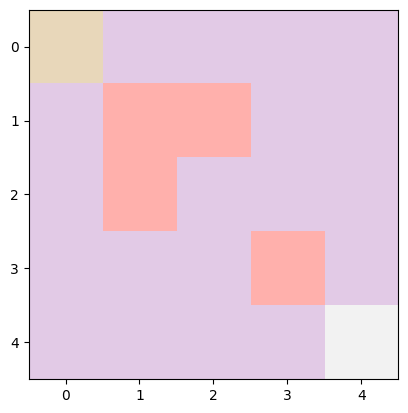
Within the setting above the top-left block is the beginning state, the bottom-right block is the objective, and the pink blocks within the center are the obstacles. Observe that the obstacles will range everytime you create an setting, as they’re generated randomly.
Producing Obstacles (generate_obstacles technique)
def generate_obstacles(self):
    for _ in vary(self.num_obstacles):
        whereas True:
            impediment = (np.random.randint(self.dimension), np.random.randint(self.dimension))
            if impediment not in self.obstacles and impediment != (0, 0) and impediment != (self.size-1, self.size-1):
                self.obstacles.append(impediment)
                  break
This technique locations num_obstacles randomly inside the grid. It ensures that obstacles don't overlap with the place to begin or the objective.
It does this by looping till the desired variety of obstacles ( self.num_obstacles)have been positioned. In each loop, it randomly selects a place within the grid, then if the place isn’t already an impediment, and never the beginning or objective, it’s added to the checklist of obstacles.
Taking a Step (step technique)
def step(self, motion):
    x, y = self.state
    if motion == 0:  # up
        x = max(0, x-1)
    elif motion == 1:  # proper
        y = min(self.size-1, y+1)
    elif motion == 2:  # down
        x = min(self.size-1, x+1)
    elif motion == 3:  # left
        y = max(0, y-1)
    self.state = (x, y)
    if self.state in self.obstacles:
        return self.state, -1, True
    if self.state == self.objective:
        return self.state, 1, True
    return self.state, -0.01, False
The step technique strikes the agent in accordance with the motion (0 for up, 1 for proper, 2 for down, 3 for left) and updates its state. It additionally checks the brand new place to see if it’s an impediment or a objective.
It does that by taking the present state (x, y), which is the present location of the agent. Then, it modifications x or y based mostly on the motion (0 for up, 1 for proper, 2 for down, 3 for left), guaranteeing the agent doesn't transfer outdoors the grid boundaries. It updates self.state to this new place. Then it checks if the brand new state is an impediment or the objective and returns the corresponding reward and whether or not the episode is completed (completed).
Resetting the Atmosphere (reset technique)
def reset(self):
    self.state = (0, 0)
    return self.state
This operate places the agent again at the place to begin. It's used in the beginning of a brand new studying episode.
It merely units self.state again to (0, 0) and returns this as the brand new state.
4.2: The Q-Studying Class
It is a Python class that represents a Q-learning agent, which can discover ways to navigate the GridWorld.
Initialization (__init__ technique)
def __init__(self, env, alpha=0.5, gamma=0.95, epsilon=0.1, episodes=10):
    self.env = env
    self.alpha = alpha
    self.gamma = gamma
    self.epsilon = epsilon
    self.episodes = episodes
    self.q_table = np.zeros((self.env.dimension, self.env.dimension, 4))
If you create a QLearning agent, you present it with the setting to study from self.env, which is the GridWorld setting in our case; a studying charge alpha, which controls how new info impacts the present Q-values; a reduction issue gamma, which determines the significance of future rewards; an exploration charge epsilon, which controls the trade-off between exploration and exploitation.
Then, we additionally initialize the variety of episodes for coaching. The Q-table, which shops the agent's data, and it’s a 3D numpy array of zeros with dimensions (env.dimension, env.dimension, 4), representing the Q-values for every state-action pair. 4 is the variety of attainable actions the agent can absorb each state.
Selecting an Motion (choose_action technique)
def choose_action(self, state):
    if np.random.uniform(0, 1) < self.epsilon:
        return np.random.alternative([0, 1, 2, 3])  # exploration
    else:
        return np.argmax(self.q_table[state])  # exploitation
The agent picks an motion based mostly on the epsilon-greedy coverage. More often than not, it chooses the best-known motion (exploitation), however generally it randomly explores different actions.
Right here, epsilon is the likelihood a random motion is chosen. In any other case, the motion with the best Q-value for the present state is chosen (argmax over the Q-values).
In our instance, we set epsilon it to 0.1, which signifies that the agent will take a random motion 10% of the time. Subsequently, when np.random.uniform(0,1) producing a quantity decrease than 0.1, a random motion will likely be taken. That is completed to forestall the agent from being caught on a suboptimal technique, and as an alternative going out and exploring earlier than being set on one.
Updating the Q-Desk (update_q_table technique)
def update_q_table(self, state, motion, reward, new_state):
    self.q_table[state][action] = (1 - self.alpha) * self.q_table[state][action] +
        self.alpha * (reward + self.gamma * np.max(self.q_table[new_state]))
After the agent takes an motion, it updates its Q-table with the brand new data. It adjusts the worth of the motion based mostly on the rapid reward and the discounted future rewards from the brand new state.
It updates the Q-table utilizing the Q-learning replace rule. It modifies the worth for the state-action pair within the Q-table (self.q_table[state][action]) based mostly on the obtained reward and the estimated future rewards (utilizing np.max(self.q_table[new_state]) for the long run state).
Coaching the Agent (prepare technique)
def prepare(self):
    rewards = []
    states = []  # Retailer states at every step
    begins = []  # Retailer the beginning of every new episode
    steps_per_episode = []  # Retailer the variety of steps per episode
    steps = 0  # Initialize the step counter outdoors the episode loop
    episode = 0
    whereas episode < self.episodes:
        state = self.env.reset()
        total_reward = 0
        completed = False
        whereas not completed:
            motion = self.choose_action(state)
            new_state, reward, completed = self.env.step(motion)
            self.update_q_table(state, motion, reward, new_state)
            state = new_state
            total_reward += reward
            states.append(state)  # Retailer state
            steps += 1  # Increment the step counter
            if completed and state == self.env.objective:  # Examine if the agent has reached the objective
                begins.append(len(states))  # Retailer the beginning of the brand new episode
                rewards.append(total_reward)
                steps_per_episode.append(steps)  # Retailer the variety of steps for this episode
                steps = 0  # Reset the step counter
                episode += 1
    return rewards, states, begins, steps_per_episode
This operate is fairly simple, it runs the agent via many episodes utilizing some time loop. In each episode, it first resets the setting by inserting the agent within the beginning state (0,0). Then, it chooses actions, updates the Q-table, and retains observe of the whole rewards and steps it takes.
Saving and Loading the Q-Desk (save_q_table and load_q_table strategies)
def save_q_table(self, filename):
    filename = os.path.be part of(os.path.dirname(__file__), filename)
    with open(filename, 'wb') as f:
        pickle.dump(self.q_table, f)

def load_q_table(self, filename):
    filename = os.path.be part of(os.path.dirname(__file__), filename)
    with open(filename, 'rb') as f:
        self.q_table = pickle.load(f)
These strategies are used to avoid wasting the realized Q-table to a file and cargo it again. They use the pickle module to serialize (pickle.dump) and deserialize (pickle.load) the Q-table, permitting the agent to renew studying with out ranging from scratch.
Operating the Simulation
Lastly, the script initializes the setting and the agent, optionally masses an current Q-table, after which begins the coaching course of. After coaching, it saves the up to date Q-table. There’s additionally a visualization part that reveals the agent shifting via the grid, which helps you see what the agent has realized.
Initialization
Firstly, the setting and agent are initialized:
env = GridWorld(dimension=5, num_obstacles=5)
agent = QLearning(env)
Right here, a GridWorld of dimension 5×5 with 5 obstacles is created. Then, a QLearning agent is initialized utilizing this setting.
Loading and Saving the Q-table
If there’s a Q-table file already saved ('q_table.pkl'), it's loaded, which permits the agent to proceed studying from the place it left off:
if os.path.exists(os.path.be part of(os.path.dirname(__file__), 'q_table.pkl')):
    agent.load_q_table('q_table.pkl')
After the agent is skilled for the desired variety of episodes, the up to date Q-table is saved:
agent.save_q_table('q_table.pkl')
This ensures that the agent’s studying isn’t misplaced and can be utilized in future coaching periods or precise navigation duties.
Coaching the Agent
The agent is skilled by calling the prepare technique, which runs via the desired variety of episodes, permitting the agent to discover the setting, replace its Q-table, and observe its progress:
rewards, states, begins, steps_per_episode = agent.prepare()
Throughout coaching, the agent chooses actions, updates the Q-table, observes rewards, and retains observe of states visited. All of this info is used to regulate the agent’s coverage (i.e., the Q-table) to enhance its decision-making over time.
Visualization

After coaching, the code makes use of matplotlib to create an animation displaying the agent’s journey via the grid. It visualizes how the agent strikes, the place the obstacles are, and the trail to the objective:
fig, ax = plt.subplots()
def replace(i):
    # Replace the grid visualization based mostly on the agent's present state
    ax.clear()
    # Calculate the cumulative reward as much as the present step
    cumulative_reward = sum(rewards[:i+1])
    # Discover the present episode
    current_episode = subsequent((j for j, begin in enumerate(begins) if begin > i), len(begins)) - 1
    # Calculate the variety of steps because the begin of the present episode
    if current_episode < 0:
        steps = i + 1
    else:
        steps = i - begins[current_episode] + 1
    ax.set_title(f"Iteration: {current_episode+1}, Complete Reward: {cumulative_reward:.2f}, Steps: {steps}")
    grid = np.zeros((env.dimension, env.dimension))
    for impediment in env.obstacles:
        grid[obstacle] = -1
    grid[env.goal] = 1
    grid[states[i]] = 0.5  # Use states[i] as an alternative of env.state
    ax.imshow(grid, cmap='cool')
ani = animation.FuncAnimation(fig, replace, frames=vary(len(states)), repeat=False)
plt.present()
This visualization isn’t solely a pleasant technique to see what the agent has realized, however it additionally offers perception into the agent’s habits and decision-making course of.
By operating this simulation a number of occasions (as indicated by the loop for i in vary(10):), the agent can have a number of studying periods, which might probably result in improved efficiency because the Q-table will get refined with every iteration.
Now do that code out, and test what number of steps it takes for the agent to achieve the objective by iteration. Moreover, attempt to improve the scale of the setting, and see how this impacts the efficiency.
5: Subsequent Steps and Future Instructions
As we take a step again to guage our journey with Q-learning and the GridWorld setup, it’s essential to understand our progress but in addition to notice the place we hit snags. Positive, we’ve bought our brokers shifting round a fundamental setting, however there are a bunch of hurdles we nonetheless want to leap over to kick their expertise up a notch.
5.1: Present Issues and Limitations
Restricted Complexity
Proper now, GridWorld is fairly fundamental and doesn’t fairly match as much as the messy actuality of the world round us, which is filled with unpredictable twists and turns.
Scalability Points
After we attempt to make the setting larger or extra advanced, our Q-table (our cheat sheet of kinds) will get too cumbersome, making Q-learning sluggish and a troublesome nut to crack.
One-Measurement-Matches-All Rewards
We’re utilizing a easy reward system — dodging obstacles shedding factors, and reaching the objective and gaining factors. However we’re lacking out on the nuances, like various rewards for various actions that would steer the agent extra subtly.
Discrete Actions and States
Our present Q-learning vibe works with clear-cut states and actions. However life’s not like that; it’s filled with shades of gray, requiring extra versatile approaches.
Lack of Generalization
Our agent learns particular strikes for particular conditions with out getting the knack for winging it in situations it hasn’t seen earlier than or making use of what it is aware of to completely different however comparable duties.
5.2: Subsequent Steps
Coverage Gradient Strategies
Coverage gradient strategies symbolize a category of algorithms in reinforcement studying that optimize the coverage immediately. They’re significantly well-suited for issues with:
- Excessive-dimensional or steady motion areas.
- The necessity for fine-grained management over the actions.
- Advanced environments the place the agent should study extra summary ideas.
The following article will cowl every little thing mandatory to know and implement coverage gradient strategies.
We’ll begin with the conceptual underpinnings of coverage gradient strategies, explaining how they differ from value-based approaches and their benefits.
We’ll dive into algorithms like REINFORCE and Actor-Critic strategies, exploring how they work and when to make use of them. We’ll focus on the exploration methods utilized in coverage gradient strategies, that are essential for efficient studying in advanced environments.
A key problem with coverage gradients is excessive variance within the updates. We are going to look into strategies like baselines and benefit capabilities to deal with this subject.
A Extra Advanced Atmosphere
To actually harness the facility of coverage gradient strategies, we are going to introduce a extra advanced setting. This setting can have a steady state and motion house, presenting a extra life like and difficult studying situation. A number of paths to success, require the agent to develop nuanced methods. The potential for extra dynamic parts, equivalent to shifting obstacles or altering objectives.
Keep tuned as we put together to embark on this thrilling journey into the world of coverage gradient strategies, the place we’ll empower our brokers to deal with challenges of accelerating complexity and nearer to real-world functions.
6: Conclusion
As we conclude this text, it’s clear that the journey via the basics of reinforcement studying has set a sturdy stage for our subsequent foray into the sphere. We’ve seen our agent begin from scratch, studying to navigate the easy corridors of the GridWorld, and now it stands on the point of stepping right into a world that’s richer and extra reflective of the complexities it should grasp.
It was rather a lot, however you made it to the top. Congrats! I hope you loved this text. In that case think about leaving a clap and following me, as I’ll often publish comparable articles. Let me know what you consider the article, what you want to see extra. Take into account leaving a clap or two and observe me to remain up to date.
Reinforcement Studying 101: Q-Studying was initially printed in In the direction of Knowledge Science on Medium, the place individuals are persevering with the dialog by highlighting and responding to this story.
[ad_2]
Supply hyperlink