


")
Skinny & Gentle Laptop computer,Intel Core i9-13900H thirteenth Gen, 16″ (40.64 cm) FHD+(16GB RAM/512GB SSD/Intel Iris Xe/Win 11/Workplace 2021/Backlit KB/Fingerprint/Black/1.88 kg) X1605VA-MB947WS")
 Lenovo Thinkpad Laptop computer X250 Intel Core i5 – 5300u Processor, 4 GB Ram & 512 GB SSD & 500GB HDD, Win10, 12.5 Inches 1.3 KG Ultralight Laptop")
, 83GS003UIN")
 Dell Latitude 5280 seventh Gen Intel Core i5 Skinny & Mild HD Laptop computer (8 GB DDR4 RAM/512 GB SSD/12.5″ (31.8 cm) HD/Home windows 11/MS Workplace/WiFi/BT/Intel UHD Graphics)")
 HP Slate 7 VoiceTab Pill (WiFi, 3G, Voice Calling), Snow White")
 Nokia T20 Tab, 8200mAh Battery, 10.36 inches 2K Display with Low Blue Gentle, Wi-Fi, 3GB RAM, 32GB storage, expandable as much as 512GB")
 Dynamic AMOLED 2X Show, RAM 12 GB, ROM 256 GB Expandable, S Pen in-Field, Wi-Fi + 5G Pill, Grey")
 Coloration Mild Brown")

 – Starlight")


")


Why the Pattern Imply Isn’t All the time the Finest
Averaging is among the most elementary instruments in statistics, second solely to counting. Whereas its simplicity may make it appear intuitive, averaging performs a central function in lots of mathematical ideas due to its sturdy properties. Main ends in likelihood, such because the Regulation of Massive Numbers and the Central Restrict Theorem, emphasize that averaging isn’t simply handy — it’s usually optimum for estimating parameters. Core statistical strategies, like Most Probability Estimators and Minimal Variance Unbiased Estimators (MVUE), reinforce this notion.
Nonetheless, this long-held perception was upended in 1956[1] when Charles Stein made a breakthrough that challenged over 150 years of estimation concept.
Historical past
Averaging has historically been seen as an efficient methodology for estimating the central tendency of a random variable’s distribution, notably within the case of a standard distribution. The traditional (or Gaussian) distribution is characterised by its bell-shaped curve and two key parameters: the imply (θ) and the usual deviation (σ). The imply signifies the middle of the curve, whereas the usual deviation displays the unfold of the information.
Statisticians usually work backward, inferring these parameters from noticed information. Gauss demonstrated that the pattern imply maximizes the chance of observing the information, making it an unbiased estimator — which means it doesn’t systematically overestimate or underestimate the true imply (θ).
Additional developments in statistical concept confirmed the utility of the pattern imply, which minimizes the anticipated squared error when in comparison with different linear unbiased estimators. Researchers like R.A. Fisher and Jerzy Neyman expanded on these concepts by introducing danger features, which measure the common squared error for various values of θ. They discovered that whereas each the imply and the median have fixed danger, the imply constantly delivers decrease danger, confirming its superiority.
Nonetheless, Stein’s theorem confirmed that when estimating three or extra parameters concurrently, the pattern imply turns into inadmissible. In these instances, biased estimators can outperform the pattern imply by providing decrease general danger. Stein’s work revolutionized statistical inference, enhancing accuracy in multi-parameter estimation.
The James-Stein Estimator
The James-Stein[2] estimator is a key software within the paradox found by Charles Stein. It challenges the notion that the pattern imply is at all times the perfect estimator, notably when estimating a number of parameters concurrently. The thought behind the James-Stein estimator is to “shrink” particular person pattern means towards a central worth (the grand imply), which reduces the general estimation error.
To make clear this, let’s begin by contemplating a vector x representing the pattern technique of a number of variables (not essentially impartial). If we take the common of all these means, we get a single worth, denoted by μ, which we confer with because the grand imply. The James-Stein estimator works by transferring every pattern imply nearer to this grand imply, lowering their variance.
The final formulation[3] for the James-Stein estimator is:
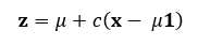
The place:
- x is the pattern imply vector.
- μ is the grand imply (the common of the pattern means).
- c is a shrinkage issue that lies between 0 and 1. It determines how a lot we pull the person means towards the grand imply.
The objective right here is to scale back the gap between the person pattern means and the grand imply. For instance, if one pattern imply is way from the grand imply, the estimator will shrink it towards the middle, smoothing out the variation within the information.
The worth of c, the shrinkage issue, will depend on the information and what’s being estimated. A pattern imply vector follows a multivariate regular distribution, so if that is what we try to estimate, the formulation turns into:
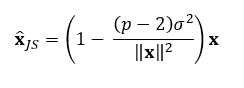
The place:
- p is the variety of parameters being estimated (the size of x).
- σ² is the variance of the pattern imply vector x.
- The time period (p — 2)/||x||² adjusts the quantity of shrinkage based mostly on the information’s variance and the variety of parameters.
Key Assumptions and Changes
One key assumption for utilizing the James-Stein estimator is that the variance σ² is similar for all variables, which is commonly not life like in real-world information. Nonetheless, this assumption could be mitigated by standardizing the information, so all variables have the identical variance. Alternatively, you’ll be able to common the person variances into one pooled estimate. This strategy works particularly nicely with bigger datasets, the place the variance variations are inclined to diminish as pattern dimension will increase.
As soon as the information is standardized or pooled, the shrinkage issue could be utilized to regulate every pattern imply appropriately.
Selecting the Shrinkage Issue
The shrinkage issue c is essential as a result of it controls how a lot the pattern means are pulled towards the grand imply. A price of c near 1 means little to no shrinkage, which resembles the conduct of the common pattern imply. Conversely, a c near 0 means vital shrinkage, pulling the pattern means virtually completely towards the grand imply.
The optimum worth of c will depend on the precise information and the parameters being estimated, however the normal guideline is that the extra parameters there are (i.e., bigger p), the extra shrinkage is helpful, as this reduces the danger of over becoming to noisy information.
Implementing the James-Stein Estimator in Code
Listed here are the James-Stein estimator features in R, Python, and Julia:
## R ##
james_stein_estimator <- operate(Xbar, sigma2 = 1) {
  p <- size(Xbar)
  norm_X2 <- sum(Xbar^2)
  shrinkage_factor <- max(0, 1 - (p - 2) * imply(sigma2) / norm_X2)
  return(shrinkage_factor * Xbar)
}

## Python ##
import numpy as np

def james_stein_estimator(Xbar, sigma2=1):
    p = len(Xbar)
    norm_X2 = np.sum(Xbar**2)
    shrinkage_factor = max(0, 1 - (p - 2) * np.imply(sigma2) / norm_X2)
    return shrinkage_factor * Xbar

## Julia ##
operate james_stein_estimator(Xbar, sigma2=1)
    p = size(Xbar)
    norm_X2 = sum(Xbar.^2)
    shrinkage_factor = max(0, 1 - (p - 2) * imply(sigma2) / norm_X2)
    return shrinkage_factor * Xbar
finish
Instance
To show the flexibility of this system, I’ll generate a 6-dimensional information set with every column containing numerical information from numerous random distributions. Listed here are the precise distributions and parameters of every I can be utilizing:
X1 ~ t-distribution (ν = 3)
X2 ~ Binomial (n = 10, p = 0.4)
X3 ~ Gamma (α = 3, β = 2)
X4 ~ Uniform (a = 0, b = 1)
X5 ~ Exponential (λ = 50)
X6 ~ Poisson (λ = 2)
Word every column on this information set incorporates impartial variables, in that no column must be correlated with one other since they had been created independently. This isn’t a requirement to make use of this methodology. It was carried out this manner merely for simplicity and to show the paradoxical nature of this consequence. In the event you’re not completely accustomed to all or any of those distributions, I’ll embrace a easy visible of every of the univariate columns of the randomly generated information. That is merely one iteration of 1,000 generated random variables from every of the aforementioned distributions.
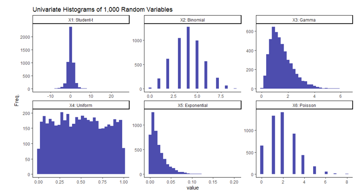
It must be clear from the histograms above that not all of those variables comply with a standard distribution implying the dataset as a complete is just not multivariate regular.
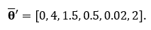
For the reason that true distributions of every are recognized, we all know the true averages of every. The typical of this multivariate dataset could be expressed in vector type with every row entry representing the common of the variable respectively. On this instance,
Realizing the true averages of every variable will enable us to have the ability to measure how shut the pattern imply, or James Stein estimator will get implying the nearer the higher. Beneath is the experiment I ran in R code which generated every of the 6 random variables and examined towards the true averages utilizing the Imply Squared Error. This experiment was then ran 10,000 instances utilizing 4 completely different pattern sizes: 5, 50, 500, and 5,000.
set.seed(42)
## Perform to calculate Imply Squared Error ##
mse <- operate(x, true_value)
  return( imply( (x - true_value)^2 ) )
## True Common ##
mu <- c(0, 4, 1.5, 0.5, 0.02, 2)
## Retailer Common and J.S. Estimator Errors ##
Xbar.MSE <- checklist(); JS.MSE <- checklist()
for(n in c(5, 50, 500, 5000)){ # Testing pattern sizes of 5, 30, 200, and 5,000
  for(i in 1:1e4){ # Performing 10,000 iterations

    ## Six Random Variables ##
    X1 <- rt(n, df = 3)
    X2 <- rbinom(n, dimension = 10, prob = 0.4)
    X3 <- rgamma(n, form = 3, fee = 2)
    X4 <- runif(n)
    X5 <- rexp(n, fee = 50)
    X6 <- rpois(n, lambda = 2)

    X <- cbind(X1, X2, X3, X4, X5, X6)

    ## Estimating Std. Dev. of Every and Standardizing Information ##
    sigma <- apply(X, MARGIN = 2, FUN = sd)

    ## Pattern Imply ##
    Xbar <- colMeans(X)

    ## J.S. Estimator ##
    JS.Xbar <- james_stein_estimator(Xbar=Xbar, sigma2=sigma/n)

    Xbar.MSE[[as.character(n)]][i] <- mse(Xbar, mu)
    JS.MSE[[as.character(n)]][i] <- mse(JS.Xbar, mu)

  }
}
sapply(Xbar.MSE, imply) # Avg. Pattern Imply MSE
sapply(JS.MSE, imply) # Avg. James-Stein MSE
From all 40,000 trails, the entire common MSE of every pattern dimension is computed by working the final two traces. The outcomes of every could be seen within the desk beneath.
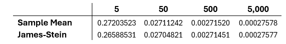
The outcomes of this of this simulation present that the James-Stein estimator is constantly higher than the pattern imply utilizing the MSE, however that this distinction decreases because the pattern dimension will increase.
Conclusion
The James-Stein estimator demonstrates a paradox in estimation: it’s attainable to enhance estimates by incorporating data from seemingly impartial variables. Whereas the distinction in MSE is likely to be negligible for big pattern sizes, this consequence sparked a lot debate when it was first launched. The invention marked a key turning level in statistical concept, and it stays related at present for multi-parameter estimation.
In the event you’d wish to discover extra, try this detailed article on Stein’s paradox and different references used to put in writing this doc.
References
[1] Stein, C. (1956). Inadmissibility of the standard estimator for the imply of a multivariate regular distribution. Proceedings of the Third Berkeley Symposium on Mathematical Statistics and Likelihood, 1, 197–206.
[2] Stein, C. (1961). Estimation with quadratic loss. In S. S. Gupta & J. O. Berger (Eds.), Statistical Resolution Principle and Associated Matters (Vol. 1, pp. 361–379). Tutorial Press.
[3] Efron, B., & Morris, C. (1977). Stein’s paradox in statistics. Scientific American, 236(5), 119–127
Stein’s Paradox was initially revealed in In the direction of Information Science on Medium, the place persons are persevering with the dialog by highlighting and responding to this story.