


")


Exploring the foundations, ideas, and math of kernel density estimation
The Kernel Density Estimator is a basic non-parametric technique that may be a versatile software for uncovering the hidden distributions of your knowledge. This text delves into the mathematical foundations of the estimator, gives steerage on selecting the optimum bandwidth, and briefly touches on the selection of kernel features and different associated matters.
Half 1: Introduction
Suppose I provide the following pattern of knowledge:
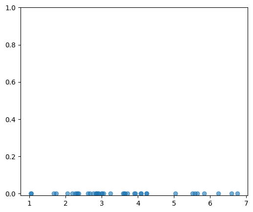
One of many first and best steps in analyzing pattern knowledge is to generate a histogram, for our knowledge we get the next:
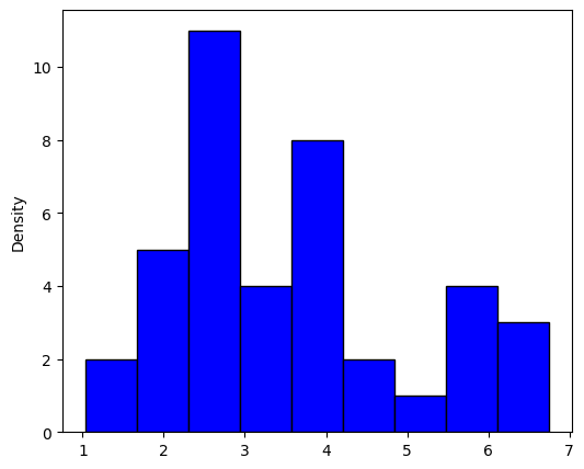
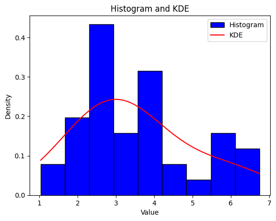
Not very helpful, and we aren’t any nearer to understanding what the underlying distribution is. There may be additionally the extra downside that, in observe, knowledge not often exhibit the sharp rectangular construction produced by a histogram. The kernel density estimator gives a treatment, and it’s a non-parametric solution to estimate the likelihood density perform of a random variable.
import numpy as np
import matplotlib.pyplot as plt
from sklearn.neighbors import KernelDensity

# Generate pattern knowledge
np.random.seed(14)
uniform_data = np.random.uniform(low=1, excessive=7, measurement=20)
normal_data = np.random.regular(loc=3, scale=0.7, measurement=20)

# Mix each distributions
combined_data = np.concatenate([uniform_data, normal_data])

# Compute histogram
hist, bin_edges = np.histogram(combined_data, bins=9, density=True)

# Compute KDE
kde = KernelDensity(kernel='gaussian').match(combined_data[:, None])
x = np.linspace(min(combined_data), max(combined_data), 1000)[:, None]
log_density = kde.score_samples(x)
density = np.exp(log_density)

# Plot histogram
plt.hist(combined_data, bins=9, density=True, shade='blue', edgecolor='black', label='Histogram')

# Plot KDE
plt.plot(x, density, shade='crimson', label='KDE')

# Add labels and legend
plt.ylabel('Density')
plt.title('Histogram and KDE')
plt.legend()

# Present plot
plt.present()
Half 2: Derivation
The next derivation takes inspiration from Bruce E. Hansen’s “Lecture Notes on Nonparametric” (2009). If you’re eager about studying extra you’ll be able to consult with his authentic lecture notes right here.
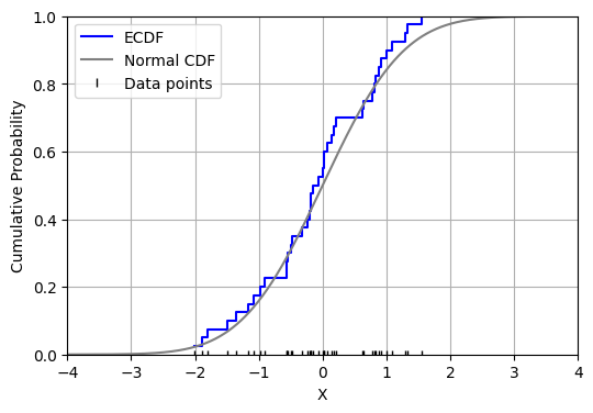
Suppose we needed to estimate a likelihood density perform, f(t), from a pattern of information. A great beginning place can be to estimate the cumulative distribution perform, F(t), utilizing the empirical distribution perform (EDF). Let X1, …, Xn be unbiased, identically distributed actual random variables with the frequent cumulative distribution perform F(t). The EDF is outlined as:

Then, by the robust legislation of enormous numbers, as n approaches infinity, the EDF converges nearly certainly to F(t). Now, the EDF is a step perform that would seem like the next:
import numpy as np
import matplotlib.pyplot as plt
from scipy.stats import norm

# Generate pattern knowledge
np.random.seed(14)
knowledge = np.random.regular(loc=0, scale=1, measurement=40)

# Type the info
data_sorted = np.kind(knowledge)

# Compute ECDF values
ecdf_y = np.arange(1, len(data_sorted)+1) / len(data_sorted)

# Generate x values for the traditional CDF
x = np.linspace(-4, 4, 1000)
cdf_y = norm.cdf(x)

# Create the plot
plt.determine(figsize=(6, 4))
plt.step(data_sorted, ecdf_y, the place='put up', shade='blue', label='ECDF')
plt.plot(x, cdf_y, shade='grey', label='Regular CDF')
plt.plot(data_sorted, np.zeros_like(data_sorted), '|', shade='black', label='Knowledge factors')

# Label axes
plt.xlabel('X')
plt.ylabel('Cumulative Likelihood')

# Add grid
plt.grid(True)

# Set limits
plt.xlim([-4, 4])
plt.ylim([0, 1])

# Add legend
plt.legend()

# Present plot
plt.present()
Subsequently, if we had been to try to discover an estimator for f(t) by taking the spinoff of the EDF, we’d get a scaled sum of Dirac delta features, which isn’t very useful. As a substitute allow us to think about using the two-point central distinction components of the estimator as an approximation of the spinoff. Which, for a small h>0, we get:
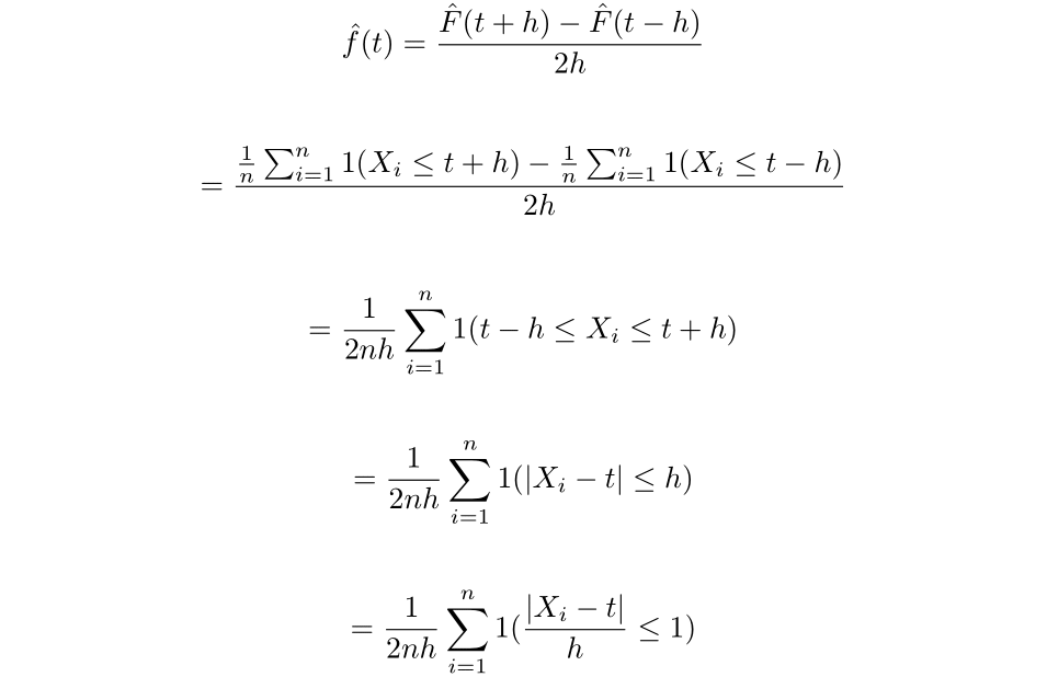
Now outline the perform okay(u) as follows:

Then we now have that:

Which is a particular case of the kernel density estimator, the place right here okay is the uniform kernel perform. Extra typically, a kernel perform is a non-negative perform from the reals to the reals which satisfies:

We are going to assume that every one kernels mentioned on this article are symmetric, therefore we now have that okay(-u) = okay(u).
The second of a kernel, which supplies insights into the form and habits of the kernel perform, is outlined as the next:

Lastly, the order of a kernel is outlined as the primary non-zero second.
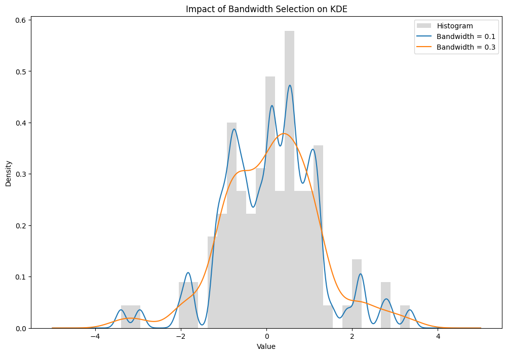
We will solely reduce the error of the kernel density estimator by both altering the h worth (bandwidth), or the kernel perform. The bandwidth parameter has a a lot bigger affect on the ensuing estimate than the kernel perform however can be way more troublesome to decide on. To reveal the affect of the h worth, take the next two kernel density estimates. A Gaussian kernel was used to estimate a pattern generated from an ordinary regular distribution, the one distinction between the estimators is the chosen h worth.
import numpy as np
import matplotlib.pyplot as plt
from scipy.stats import gaussian_kde

# Generate pattern knowledge
np.random.seed(14)
knowledge = np.random.regular(loc=0, scale=1, measurement=100)

# Outline the bandwidths
bandwidths = [0.1, 0.3]

# Plot the histogram and KDE for every bandwidth
plt.determine(figsize=(12, 8))
plt.hist(knowledge, bins=30, density=True, shade='grey', alpha=0.3, label='Histogram')

x = np.linspace(-5, 5, 1000)
for bw in bandwidths:
    kde = gaussian_kde(knowledge , bw_method=bw)
    plt.plot(x, kde(x), label=f'Bandwidth = {bw}')

# Add labels and title
plt.title('Influence of Bandwidth Choice on KDE')
plt.xlabel('Worth')
plt.ylabel('Density')
plt.legend()
plt.present()
Fairly a dramatic distinction.
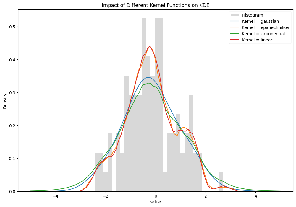
Now allow us to take a look at the affect of fixing the kernel perform whereas protecting the bandwidth fixed.
import numpy as np
import matplotlib.pyplot as plt
from sklearn.neighbors import KernelDensity

# Generate pattern knowledge
np.random.seed(14)
knowledge = np.random.regular(loc=0, scale=1, measurement=100)[:, np.newaxis]  # reshape for sklearn

# Intialize a relentless bandwidth
bandwidth = 0.6

# Outline totally different kernel features
kernels = ["gaussian", "epanechnikov", "exponential", "linear"]

# Plot the histogram (clear) and KDE for every kernel
plt.determine(figsize=(12, 8))

# Plot the histogram
plt.hist(knowledge, bins=30, density=True, shade="grey", alpha=0.3, label="Histogram")

# Plot KDE for every kernel perform
x = np.linspace(-5, 5, 1000)[:, np.newaxis]
for kernel in kernels:
    kde = KernelDensity(bandwidth=bandwidth, kernel=kernel)
    kde.match(knowledge)
    log_density = kde.score_samples(x)
    plt.plot(x[:, 0], np.exp(log_density), label=f"Kernel = {kernel}")

plt.title("Influence of Totally different Kernel Features on KDE")
plt.xlabel("Worth")
plt.ylabel("Density")
plt.legend()
plt.present()
Whereas visually there’s a massive distinction within the tails, the general form of the estimators are comparable throughout the totally different kernel features. Subsequently, I’ll focus primarily give attention to discovering the optimum bandwidth for the estimator. Now, let’s discover among the properties of the kernel density estimator, together with its bias and variance.
Half 3: Properties of the Kernel Density Estimator
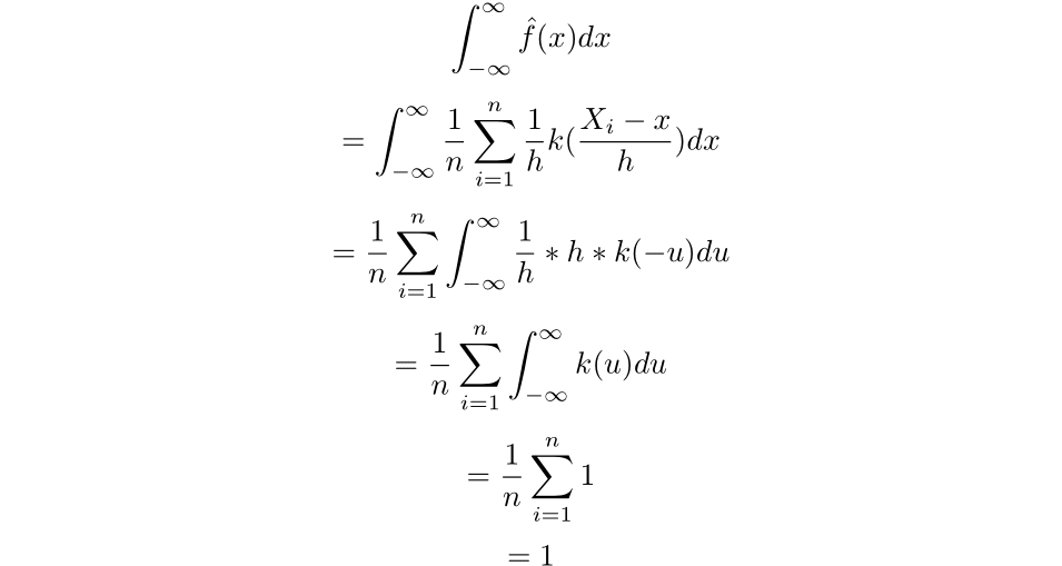
The primary indisputable fact that we might want to make the most of is that the integral of the estimator throughout the true line is 1. To show this truth, we might want to make use of the change of u-substitution:

Using that u-substitution we get the next:
Now we will discover the imply of the estimated density:
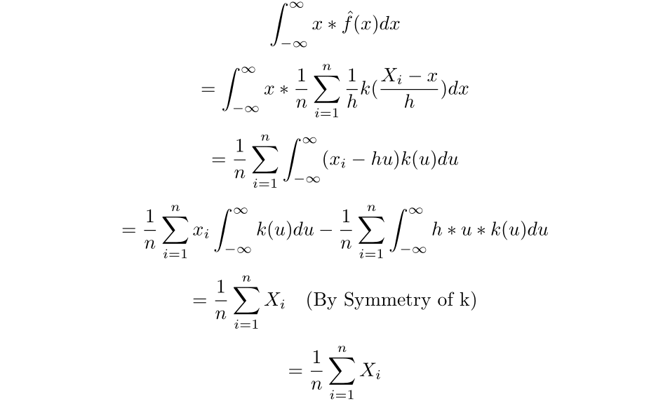
Subsequently, the imply of the estimated density is solely the pattern imply.
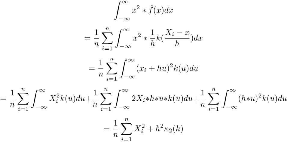
Now allow us to discover the second second of the estimator.
We will then discover the variance of the estimated density:

To seek out the optimum bandwidth and kernel, we shall be minimizing the imply squared error of the estimator. To realize this, we’ll first want to search out the bias and variance of the estimator.
The anticipated worth of a random variable, X, with a likelihood density perform of f, could be calculated as:

Thus,

The place z is a dummy variable of integration. We will then use a change of variables to get the next:

Subsequently, we get the next:

More often than not, nonetheless, the integral above will not be analytically solvable. Subsequently, we should approximate f(x+ hu) through the use of its Taylor enlargement. As a reminder, the Taylor enlargement of f(x) round a is:

Thus, assume f(x) is differentiable to the v+1 time period. For f(x+hu) the enlargement is:

Then for a v-order kernel, we will take the expression out to the v’th time period:

The place the final time period is the rest, which vanishes sooner than h as h approaches 0. Now, assuming that okay is a v’th order kernel perform, we now have that:

Subsequently:

Thus we now have that the bias of the estimator is then:

The higher certain for the variance could be obtained by way of the next calculation [Chen 2].
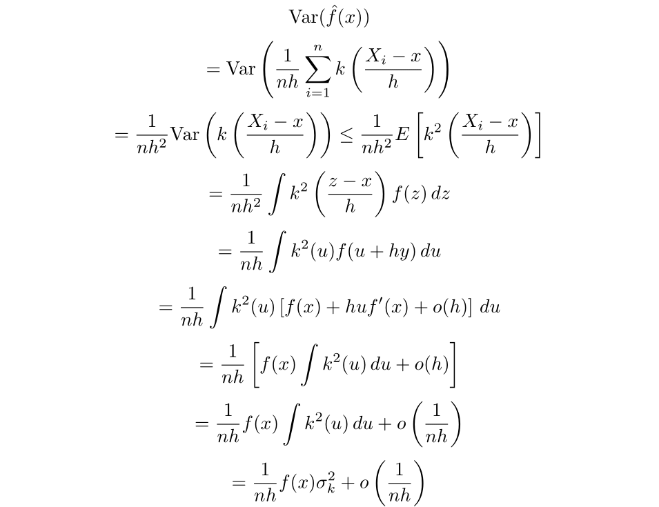
The place:

This time period is also referred to as the roughness and could be denoted as R(okay).
Lastly, we will get an expression for the imply squared error:
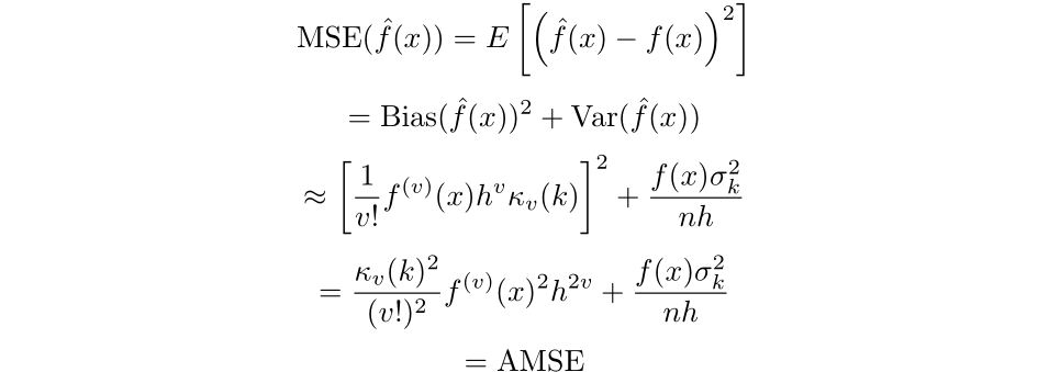
The place AMSE is brief for asymptotic imply squared error. We will then reduce the asymptotic imply built-in sq. error outlined as follows,

to search out what bandwidth will result in the bottom error (Silverman, 1986):

Then, by setting the equation to 0 and simplifying we discover that the optimum bandwidth for a kernel of order v is:

The extra acquainted expression is for second order kernels, the place the bandwidth that minimizes the AMISE is:

Nevertheless, this resolution could also be a letdown as we require understanding the distribution that we’re estimating to search out the optimum bandwidth. In observe, we’d not have this distribution if we had been utilizing the kernel density estimator within the first place.
Half 4: Bandwidth Choice
Regardless of not having the ability to discover the bandwidth that minimizes the imply built-in sq. error, there are a number of strategies accessible to decide on a bandwidth with out understanding the underlying distribution. You will need to notice, nonetheless, {that a} bigger h worth will trigger your estimator to have much less variance however better bias, whereas a smaller bandwidth will produce a rougher estimate with much less bias (Eidous et al., 2010).
Some strategies to discover a bandwidth embody utilizing:
1: The Clear up-the-Equation Rule
2: Least Squares Cross-Validation
3: Biased Cross-Validation
4: The Direct Plug in Technique
5: The Distinction Technique
You will need to notice that relying on the pattern measurement and skewness of your knowledge, the ‘finest’ technique to decide on your bandwidth adjustments. Most packages in Python permit you to use Silverman's proposed technique, the place you instantly plug in some distribution (sometimes regular) for f after which compute the bandwidth based mostly upon the kernel perform that you’ve got chosen. This process, often called Silverman’s Rule of Thumb, gives a comparatively easy estimate for the bandwidth. Nevertheless, it typically tends to overestimate, leading to a smoother estimate with decrease variance however greater bias. Silverman’s Rule of Thumb additionally particularly doesn’t carry out nicely for bimodal distributions, and there are extra correct strategies accessible for these instances.
In case you assume that your knowledge is often distributed with a imply of 0, use the pattern commonplace deviation, and apply the Epanechnikov kernel (mentioned beneath), you’ll be able to choose the bandwidth utilizing the Rule of Thumb by way of the next equation:

Eidous et al. discovered the Distinction Technique to have the perfect efficiency in comparison with the opposite strategies I listed. Nevertheless, this technique has drawbacks, because it will increase the variety of parameters to be chosen.
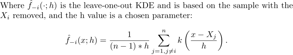
The cross validation technique is one other good selection in bandwidth choice technique, because it typically results in a small bias however a big variance (Heidenreich et al, 2013). It’s most helpful for when you’re in search of a bandwidth selector that tends to undershoot the optimum bandwidth. To maintain this text not overly lengthy I’ll solely be going over the Unusual Least Squares Cross Validation technique. The tactic tends to work nicely for relatively wiggly densities and a reasonable pattern measurement of round 50 to 100. If in case you have a really small or massive pattern measurement this paper is an effective useful resource to search out one other approach to decide on your bandwidth. As identified by Heidenreich, “it undoubtedly makes a distinction which bandwidth selector is chosen; not solely in numerical phrases but in addition for the standard of density estimation”.
As a fast refresher, after we are making a mannequin we reserve a few of our pattern as a validation set to see how our mannequin performs on the pattern that it has not been skilled on. Ok Fold Cross Validation minimizes the affect of probably choosing a take a look at set that misrepresents the dataset by splitting the dataset into Ok elements after which coaching the mannequin Ok occasions and permitting every half to be the validation set as soon as.
Depart One Out Cross Validation is Ok Fold Cross Validation taken to the intense, the place for a pattern measurement of n, we prepare the mannequin n occasions and miss one pattern every time. Right here is an article that goes extra in-depth into the strategy within the context of coaching machine studying algorithms.
Allow us to flip again to the AMISE expression. As a substitute of investigating the asymptotic imply built-in sq. error, we’ll reduce the imply built-in sq. error (MISE). First, we will increase the sq.:
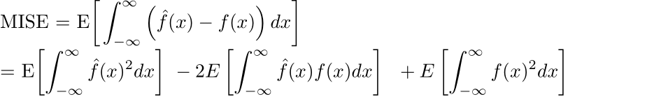
As we now have no management over the anticipated worth of the final time period, we will search to attenuate the primary two phrases and drop the third. Then, as a result of X is an unbiased estimator for E[X], we will discover the primary time period instantly:

Then the convolution of okay with okay is outlined as the next:

Therefore,

Thus, for the primary time period, we have:

Subsequent, we will approximate the second time period by Monte Carlo strategies. First, as mentioned earlier, the density perform is equal to the spinoff of the cumulative distribution perform, which we will approximate by way of the empirical distribution perform. Then, the integral could be approximated by the common worth of the estimator over the pattern.

Then the least squares cross validation selector (LSCV) is outlined as the next:

We then get the ultimate selector outlined as:
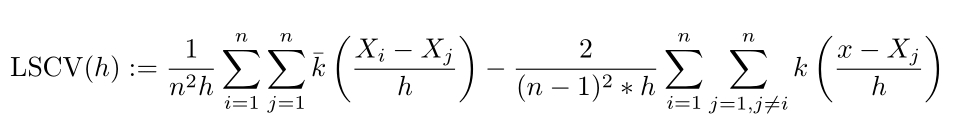
The optimum bandwidth is the h worth that minimizes LSCV, outlined as the next:

The LSCV(h) perform can have a number of native minimums, therefore the optimum bandwidth that you just discover could be delicate to the interval chosen. It’s helpful to graph the perform after which visually examine the place the worldwide minimal lies.
Half 5: Optimum Kernel Choice
If we’re working with a second order kernel (which is typical), the selection in kernel choice is way more simple than bandwidth. Below the factors of minimizing the AMISE, the Epanechnikov kernel is an optimum kernel. The total proof could be discovered on this paper by Muler.

There are different kernels that are as environment friendly because the Epanechnikov kernel, that are additionally touched on in Muler’s paper. Nevertheless, I wouldn’t fear an excessive amount of about your selection of kernel perform, the selection in bandwidth is way more vital.
Half 6: Additional Matters and Conclusion
Adaptive Bandwidths
One of many proposed methods to enhance the Kernel Density Estimator is thru an adaptive bandwidth. An adaptive bandwidth adjusts the bandwidth for every knowledge level, growing it when the density of the pattern knowledge is decrease and reducing it when the density is greater. Whereas promising in concept, an adaptive bandwidth has been proven to carry out fairly poorly within the univariate case (Terrel, Scott 1992). Whereas it might be higher for bigger dimensional areas, for the one-dimensional case I imagine it’s best to stay with a relentless bandwidth.
Multivariate Kernel Density Estimation
The kernel density estimator may also be prolonged to greater dimensions, the place the kernel is a radial foundation perform or is a product of a number of kernel features. The method does undergo from the curse of dimensionality, the place because the dimension grows bigger the variety of knowledge factors wanted to supply a helpful estimator grows exponentially. It is usually computationally costly and isn’t an excellent technique for analyzing high-dimensional knowledge.
Nonparametric multivariate density estimation continues to be a really lively subject, with Masked Autoregressive Circulate showing to be fairly a brand new and promising method.
Actual World Purposes
Kernel density estimation has quite a few functions throughout disciplines. First, it has been proven to enhance machine studying algorithms comparable to within the case of the versatile naive Bayes classifier.
It has additionally been used to estimate visitors accident density. The linked paper makes use of the KDE to assist make a mannequin that signifies the chance of visitors accidents in several cities throughout Japan.
One other enjoyable use is in seismology, the place the KDE has been used for modelling the chance of earthquakes in several places.
Conclusion
The kernel density estimator is a superb addition to the info analysts’ toolbox. Whereas a histogram is definitely a superb approach of analyzing knowledge with out utilizing any underlying assumptions, the kernel density estimator gives a stable different for univariate knowledge. For greater dimensional knowledge, or for when computational time is a priority, I’d suggest trying elsewhere. Nonetheless, the KDE is an intuitive, highly effective and versatile software in knowledge evaluation.
Until in any other case famous, all photos are by the writer.
The Math Behind Kernel Density Estimation was initially revealed in In direction of Knowledge Science on Medium, the place individuals are persevering with the dialog by highlighting and responding to this story.