Is Much less Extra? Do Deep Studying Forecasting Fashions Want Characteristic Discount?

To curate, or to not curate, that’s the query

Time sequence forecasting is a robust device in knowledge science, providing insights into future tendencies primarily based on historic patterns. In our earlier article, we explored how making your time sequence stationary mechanically can considerably improve mannequin efficiency. However stationarity is only one piece of the puzzle. As we proceed to refine our forecasting fashions, one other essential query arises: how can we deal with the multitude of options our knowledge might current?

As you’re employed with time sequence knowledge, you’ll usually end up with many potential options to incorporate in your mannequin. Whereas it’s tempting to make use of all obtainable knowledge, including extra options isn’t all the time higher. It might make your mannequin extra complicated and slower to coach, with out essentially enhancing its efficiency.

You is likely to be questioning: is it necessary to simplify the characteristic set and what are the strategies obtainable on the market? That’s precisely what we’ll focus on on this article.

Right here’s a fast abstract of what’s going to be coated:

• Characteristic discount in time sequence — We’ll clarify the idea of characteristic discount in time sequence evaluation and why it issues.
• Sensible implementation information — Utilizing Python, we’ll stroll via evaluating and deciding on options on your time sequence mannequin, offering hands-on instruments to optimize your method. We’ll additionally assess whether or not trimming down options is important for our forecasting fashions.

When you’re acquainted with strategies like stationarity and have discount as defined on this article, and also you’re seeking to elevate your fashions even additional? Try this text on utilizing a customized validation loss in your deep studying mannequin to get higher inventory forecasts — it’s an important subsequent step!

Characteristic discount in time sequence : a easy rationalization

Characteristic discount is like cleansing up your workspace to make it simpler to seek out what you want. In time sequence evaluation, it means slicing down the variety of enter variables (options) that your mannequin makes use of to make predictions. The aim is to simplify the mannequin whereas retaining its predictive energy. That is necessary as a result of too many and correlated options could make your mannequin sophisticated, gradual, and fewer correct.

Particularly, simplifying the characteristic set can :

• Decreased complexity: Fewer options means a less complicated mannequin, which is commonly quicker to coach and use.
• Improved generalization: By eradicating noise, eliminating correlated options and specializing in key data, it helps the mannequin to study the true underlying patterns fairly than memorizing redundant data. This enhances the mannequin’s potential to generalize its predictions to completely different datasets.
• Simpler interpretation: A mannequin with fewer options is commonly simpler for people to grasp and clarify.
• Computational effectivity: Fewer options requires much less reminiscence and processing energy, which might be essential for giant datasets or real-time purposes.

It’s additionally necessary to notice that the majority time sequence packages in Python for forecasting don’t carry out characteristic discount mechanically. It is a step you usually must deal with by yourself earlier than utilizing these packages.

To higher perceive these ideas, let’s stroll via a sensible instance utilizing real-world each day knowledge from the Federal Reserve Financial Knowledge (FRED) database. We’ll skip the info retrieval course of right here, as we’ve already coated the way to get free and dependable knowledge from the FRED API in a earlier article. You will get the info we’ll be utilizing this script. When you’ve fetched the info :

• Create adata listing in your present listing

mkdir -p /path/to/current_directory/knowledge

• Copy the info in your listing

cp -R /path/to/fetcher_directory /path/to/current_directory/knowledge

Now that we’ve our knowledge, let’s dive into our characteristic discount instance.

We’ve beforehand demonstrated the way to clear the each day knowledge fetched from the FRED API in one other article, so we’ll skip that course of right here and use the processed_dataframes(listing of dataframes) that resulted from the steps outlined in that article.

import pandas as pd
import os
import warnings
warnings.filterwarnings("ignore")

def is_sp500(df):
    last_date = df['ds'].max()
    last_value = float(df.loc[df['ds'] == last_date, 'worth'].iloc[0])
    return 5400 <= last_value <= 5650

initial_model_train = None
for i, df in enumerate(processed_dataframes):
    if df['value'].isna().any():
        proceed
    if is_sp500(df):
        initial_model_train = df
        break

TRAIN_SIZE = .90
START_DATE = '2018-10-01'
END_DATE = '2024-09-05'
initial_model_train = initial_model_train.rename(columns={'worth': 'value'}).reset_index(drop=True)
initial_model_train['unique_id'] = 'SPY'
initial_model_train['price'] = initial_model_train['price'].astype(float)
initial_model_train['y'] = initial_model_train['price'].pct_change()

initial_model_train = initial_model_train[initial_model_train['ds'] > START_DATE].reset_index(drop=True)
combined_df_all = pd.concat([df.drop(columns=['ds']) for df in processed_dataframes], axis=1)
combined_df_all.columns = [f'value_{i}' for i in range(len(processed_dataframes))]
rows_to_keep = len(initial_model_train)
combined_df_all = combined_df_all.iloc[-rows_to_keep:].reset_index(drop=True)

train_size = int(len(initial_model_train)*TRAIN_SIZE)
initial_model_test = initial_model_train[train_size:]
initial_model_train = initial_model_train[:train_size]
combined_df_test = combined_df_all[train_size:]
combined_df_train = combined_df_all[:train_size]

You is likely to be questioning why we’ve divided our knowledge into coaching and testing units? The reason being to make sure that there isn’t a knowledge leakage earlier than making use of any transformation or discount method.

initial_model_data accommodates the S&P 500 each day costs (saved initially processed_dataframes), which would be the knowledge we’ll be attempting to forecast.

Then, we have to guarantee our knowledge is stationary. For an in depth rationalization on the way to mechanically make your knowledge stationary and enhance your mannequin by 20%, seek advice from this article.

import numpy as np
from statsmodels.tsa.stattools import adfuller
P_VALUE = 0.05

def replace_inf_nan(sequence):
    if np.isnan(sequence.iloc[0]) or np.isinf(sequence.iloc[0]):
        sequence.iloc[0] = 0
    masks = np.isinf(sequence) | np.isnan(sequence)
    sequence = sequence.copy()
    sequence[mask] = np.nan
    sequence = sequence.ffill()
    return sequence

def safe_convert_to_numeric(sequence):
    return pd.to_numeric(sequence, errors='coerce')

tempo_df = pd.DataFrame()
stationary_df_train = pd.DataFrame()
stationary_df_test = pd.DataFrame()

value_columns = [col for col in combined_df_all.columns if col.startswith('value_')]

transformations = ['first_diff', 'pct_change', 'log', 'identity']

def get_first_diff(numeric_series):
    return replace_inf_nan(numeric_series.diff())

def get_pct_change(numeric_series):
    return replace_inf_nan(numeric_series.pct_change())

def get_log_transform(numeric_series):
    return replace_inf_nan(np.log(numeric_series.substitute(0, np.nan)))

def get_identity(numeric_series):
    return numeric_series

for index, val_col in enumerate(value_columns):
    numeric_series = safe_convert_to_numeric(combined_df_train[val_col])
    numeric_series_all = safe_convert_to_numeric(combined_df_all[val_col])

    if numeric_series.isna().all():
        proceed

    valid_transformations = []

    tempo_df['first_diff'] = get_first_diff(numeric_series)
    tempo_df['pct_change'] = get_pct_change(numeric_series)
    tempo_df['log'] = get_log_transform(numeric_series)
    tempo_df['identity'] = get_identity(numeric_series)

    for transfo in transformations:
        tempo_df[transfo] = replace_inf_nan(tempo_df[transfo])
        sequence = tempo_df[transfo].dropna()

        if len(sequence) > 1 and never (sequence == sequence.iloc[0]).all():
            end result = adfuller(sequence)
            if end result[1] < P_VALUE:
                valid_transformations.append((transfo, end result[0], end result[1]))

    if valid_transformations:
        if any(transfo == 'identification' for transfo, _, _ in valid_transformations):
            chosen_transfo = 'identification'
        else:
            chosen_transfo = min(valid_transformations, key=lambda x: x[1])[0]

        if chosen_transfo == 'first_diff':
            stationary_df_train[val_col] = get_first_diff(numeric_series_all)
        elif chosen_transfo == 'pct_change':
            stationary_df_train[val_col] = get_pct_change(numeric_series_all)
        elif chosen_transfo == 'log':
            stationary_df_train[val_col] = get_log_transform(numeric_series_all)
        else:
            stationary_df_train[val_col] = get_identity(numeric_series_all)

    else:
        print(f"No legitimate transformation discovered for {val_col}")


stationary_df_test = stationary_df_train[train_size:]
stationary_df_train = stationary_df_train[:train_size]

initial_model_train = initial_model_train.iloc[1:].reset_index(drop=True)
stationary_df_train = stationary_df_train.iloc[1:].reset_index(drop=True)
last_train_index = stationary_df_train.index[-1]
stationary_df_test = stationary_df_test.loc[last_train_index + 1:].reset_index(drop=True)
initial_model_test = initial_model_test.loc[last_train_index + 1:].reset_index(drop=True)

Then, we are going to depend the variety of variables which have a minimum of a 95% correlation coefficient with one other variable.

CORR_COFF = .95
corr_matrix = stationary_df_train.corr().abs()
masks = np.triu(np.ones_like(corr_matrix, dtype=bool), ok=1)
high_corr = corr_matrix.the place(masks).stack()
high_corr = high_corr[high_corr >= CORR_COFF]
unique_cols = set(high_corr.index.get_level_values(0)) | set(high_corr.index.get_level_values(1))
num_high_corr_cols = len(unique_cols)

print(f"n{num_high_corr_cols}/{stationary_df_train.form[1]} variables have ≥{int(CORR_COFF*100)}% "
      f"correlation with one other variable.n")

Having 260 out of 438 variables which have a correlation of 95% or extra with a minimum of one other variable might be a problem. It signifies important multicollinearity within the dataset. This redundancy can result in a number of points:

• It complicates the mannequin with out including substantial new data
• Probably causes instability in coefficient estimates
• Will increase the chance of overfitting
• Makes interpretation of particular person variable impacts difficult

Characteristic analysis and choice

We perceive that characteristic discount might be necessary, however how can we carry out it? Which strategies ought to we use? These are the questions we’ll discover now.

The primary method we’ll look at is Principal Element Evaluation (PCA). It’s a typical and an efficient dimensionality discount method. PCA identifies linear relationships between options and retains the principal parts that designate a predetermined proportion of the variance within the authentic dataset. In our use case, we’ve set the EXPLAINED_VARIANCE threshold to 90%.

from sklearn.preprocessing import StandardScaler
from sklearn.decomposition import PCA
EXPLAINED_VARIANCE = .9
MIN_VARIANCE = 1e-10

X_train = stationary_df_train.values
scaler = StandardScaler()
X_train_scaled = scaler.fit_transform(X_train)
pca = PCA(n_components=EXPLAINED_VARIANCE, svd_solver='full')
X_train_pca = pca.fit_transform(X_train_scaled)

components_to_keep = pca.explained_variance_ > MIN_VARIANCE
X_train_pca = X_train_pca[:, components_to_keep]

pca_df_train = pd.DataFrame(
    X_train_pca,
    columns=[f'PC{i+1}' for i in range(X_train_pca.shape[1])]
)

X_test = stationary_df_test.values
X_test_scaled = scaler.rework(X_test)
X_test_pca = pca.rework(X_test_scaled)

X_test_pca = X_test_pca[:, components_to_keep]

pca_df_test = pd.DataFrame(
    X_test_pca,
    columns=[f'PC{i+1}' for i in range(X_test_pca.shape[1])]
)

print(f"nOriginal variety of options: {stationary_df_train.form[1]}")
print(f"Variety of parts after PCA: {pca_df_train.form[1]}n")

It’s a formidable: solely 76 parts out of 438 options remaining after the discount whereas protecting 90% of the variance defined! Now let’s transfer to a non-linear discount method.

The Temporal Fusion Transformers (TFT) is a complicated mannequin for time sequence forecasting. It contains the Variable Choice Community (VSN), which is a key part of the mannequin. It’s particularly designed to mechanically determine and give attention to essentially the most related options inside a dataset. It achieves this by assigning discovered weights to every enter variable, successfully highlighting which options contribute most to the predictive activity.

This VSN-based method will likely be our second discount method. We’ll implement it utilizing PyTorch Forecasting, which permits us to leverage the Variable Choice Community from the TFT mannequin.

We’ll use a fundamental configuration. Our aim isn’t to create the highest-performing mannequin doable, however fairly to determine essentially the most related options whereas utilizing minimal sources.

from pytorch_forecasting import TemporalFusionTransformer, TimeSeriesDataSet
from pytorch_forecasting.metrics import QuantileLoss
from lightning.pytorch.callbacks import EarlyStopping
import lightning.pytorch as pl
import torch

pl.seed_everything(42)
max_encoder_length = 32
max_prediction_length = 1
VAL_SIZE = .2
VARIABLES_IMPORTANCE = .8
model_data_feature_sel = initial_model_train.be a part of(stationary_df_train)
model_data_feature_sel = model_data_feature_sel.be a part of(pca_df_train)
model_data_feature_sel['price'] = model_data_feature_sel['price'].astype(float)
model_data_feature_sel['y'] = model_data_feature_sel['price'].pct_change()
model_data_feature_sel = model_data_feature_sel.iloc[1:].reset_index(drop=True)

model_data_feature_sel['group'] = 'spy'
model_data_feature_sel['time_idx'] = vary(len(model_data_feature_sel))

train_size_vsn = int((1-VAL_SIZE)*len(model_data_feature_sel))
train_data_feature = model_data_feature_sel[:train_size_vsn]
val_data_feature = model_data_feature_sel[train_size_vsn:]
unknown_reals_origin = [col for col in model_data_feature_sel.columns if col.startswith('value_')] + ['y']

timeseries_config = {
    "time_idx": "time_idx",
    "goal": "y",
    "group_ids": ["group"],
    "max_encoder_length": max_encoder_length,
    "max_prediction_length": max_prediction_length,
    "time_varying_unknown_reals": unknown_reals_origin,
    "add_relative_time_idx": True,
    "add_target_scales": True,
    "add_encoder_length": True
}


training_ts = TimeSeriesDataSet(
    train_data_feature,
    **timeseries_config
)

The VARIABLES_IMPORTANCE threshold is about to 0.8, which implies we'll retain options within the prime eightieth percentile of significance as decided by the Variable Choice Community (VSN). For extra details about the Temporal Fusion Transformers (TFT) and its parameters, please seek advice from the documentation.

Subsequent, we’ll practice the TFT mannequin.

if torch.cuda.is_available():
    accelerator = 'gpu'
    num_workers = 2
else :
    accelerator = 'auto'
    num_workers = 0

validation = TimeSeriesDataSet.from_dataset(training_ts, val_data_feature, predict=True, stop_randomization=True)
train_dataloader = training_ts.to_dataloader(practice=True, batch_size=64, num_workers=num_workers)
val_dataloader = validation.to_dataloader(practice=False, batch_size=64*5, num_workers=num_workers)

tft = TemporalFusionTransformer.from_dataset(
    training_ts,
    learning_rate=0.03,
    hidden_size=16,
    attention_head_size=2,
    dropout=0.1,
    loss=QuantileLoss()
)

early_stop_callback = EarlyStopping(monitor="val_loss", min_delta=1e-5, endurance=5, verbose=False, mode="min")

coach = pl.Coach(max_epochs=20,  accelerator=accelerator, gradient_clip_val=.5, callbacks=[early_stop_callback])
coach.match(
    tft,
    train_dataloaders=train_dataloader,
    val_dataloaders=val_dataloader

)

We deliberately set max_epochs=20 so the mannequin doesn’t practice too lengthy. Moreover, we carried out an early_stop_callback that halts coaching if the mannequin exhibits no enchancment for five consecutive epochs (endurance=5).

Lastly, utilizing one of the best mannequin obtained, we choose the eightieth percentile of an important options as decided by the VSN.

best_model_path = coach.checkpoint_callback.best_model_path
best_tft = TemporalFusionTransformer.load_from_checkpoint(best_model_path)

raw_predictions = best_tft.predict(val_dataloader, mode="uncooked", return_x=True)


def get_top_encoder_variables(best_tft,interpretation):
    encoder_importances = interpretation["encoder_variables"]
    sorted_importances, indices = torch.type(encoder_importances, descending=True)
    cumulative_importances = torch.cumsum(sorted_importances, dim=0)
    threshold_index = torch.the place(cumulative_importances > VARIABLES_IMPORTANCE)[0][0]
    top_variables = [best_tft.encoder_variables[i] for i in indices[:threshold_index+1]]
    if 'relative_time_idx' in top_variables:
        top_variables.take away('relative_time_idx')
    return top_variables

interpretation= best_tft.interpret_output(raw_predictions.output, discount="sum")
top_encoder_vars = get_top_encoder_variables(best_tft,interpretation)

print(f"nOriginal variety of options: {stationary_df_train.form[1]}")
print(f"Variety of options after Variable Choice Community (VSN): {len(top_encoder_vars)}n")

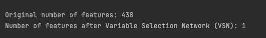
The unique dataset contained 438 options, which have been then lowered to 1 characteristic solely after making use of the VSN technique! This drastic discount suggests a number of prospects:

1. Lots of the authentic options might have been redundant.
2. The characteristic choice course of might have oversimplified the knowledge.
3. Utilizing solely the goal variable’s historic values (autoregressive method) would possibly carry out in addition to, or presumably higher than, fashions incorporating exogenous variables.

Evaluating characteristic discount strategies

On this remaining part, we evaluate out discount strategies utilized to our mannequin. Every technique is examined whereas sustaining an identical mannequin configurations, various solely the options subjected to discount.

We’ll use TiDE, a small state-of-the-art Transformer-based mannequin. We’ll use the implementation offered by NeuralForecast. Any mannequin from NeuralForecast right here would work so long as it permits exogenous historic variables.

We’ll practice and check two fashions utilizing each day SPY (S&P 500 ETF) knowledge. Each fashions can have the identical:

1. Practice-test break up ratio
2. Hyperparameters
3. Single time sequence (SPY)
4. Forecasting horizon of 1 step forward

The one distinction between the fashions would be the characteristic discount method. That’s it!

1. First mannequin: Authentic options (no characteristic discount)
2. Second mannequin: Characteristic discount utilizing PCA
3. Third mannequin: Characteristic discount utilizing VSN

This setup permits us to isolate the influence of every characteristic discount method on mannequin efficiency.

First we practice the three fashions with the identical configuration aside from the options.

from neuralforecast.fashions import TiDE
from neuralforecast import NeuralForecast

train_data = initial_model_train.be a part of(stationary_df_train)
train_data = train_data.be a part of(pca_df_train)
test_data = initial_model_test.be a part of(stationary_df_test)
test_data = test_data.be a part of(pca_df_test)

hist_exog_list_origin = [col for col in train_data.columns if col.startswith('value_')] + ['y']
hist_exog_list_pca = [col for col in train_data.columns if col.startswith('PC')] + ['y']
hist_exog_list_vsn = top_encoder_vars


tide_params = {
    "h": 1,
    "input_size": 32,
    "scaler_type": "sturdy",
    "max_steps": 500,
    "val_check_steps": 20,
    "early_stop_patience_steps": 5
}

model_original = TiDE(
    **tide_params,
    hist_exog_list=hist_exog_list_origin,
)


model_pca = TiDE(
    **tide_params,
    hist_exog_list=hist_exog_list_pca,
)

model_vsn = TiDE(
    **tide_params,
    hist_exog_list=hist_exog_list_vsn,
)

nf = NeuralForecast(
    fashions=[model_original, model_pca, model_vsn],
    freq='D'
)

val_size = int(train_size*VAL_SIZE)
nf.match(df=train_data,val_size=val_size,use_init_models=True)

Then, we make the predictions.

from tabulate import tabulate
y_hat_test_ret = pd.DataFrame()
current_train_data = train_data.copy()

y_hat_ret = nf.predict(current_train_data)
y_hat_test_ret = pd.concat([y_hat_test_ret, y_hat_ret.iloc[[-1]]])

for i in vary(len(test_data) - 1):
    combined_data = pd.concat([current_train_data, test_data.iloc[[i]]])
    y_hat_ret = nf.predict(combined_data)
    y_hat_test_ret = pd.concat([y_hat_test_ret, y_hat_ret.iloc[[-1]]])
    current_train_data = combined_data

predicted_returns_original = y_hat_test_ret['TiDE'].values
predicted_returns_pca = y_hat_test_ret['TiDE1'].values
predicted_returns_vsn = y_hat_test_ret['TiDE2'].values

predicted_prices_original = []
predicted_prices_pca = []
predicted_prices_vsn = []

for i in vary(len(predicted_returns_pca)):
    if i == 0:
        last_true_price = train_data['price'].iloc[-1]
    else:
        last_true_price = test_data['price'].iloc[i-1]
    predicted_prices_original.append(last_true_price * (1 + predicted_returns_original[i]))
    predicted_prices_pca.append(last_true_price * (1 + predicted_returns_pca[i]))
    predicted_prices_vsn.append(last_true_price * (1 + predicted_returns_vsn[i]))

true_values = test_data['price']
strategies = ['Original','PCA', 'VSN']
predicted_prices = [predicted_prices_original,predicted_prices_pca, predicted_prices_vsn]

outcomes = []

for technique, costs in zip(strategies, predicted_prices):
    mse = np.imply((np.array(costs) - true_values)**2)
    rmse = np.sqrt(mse)
    mae = np.imply(np.abs(np.array(costs) - true_values))

    outcomes.append([method, mse, rmse, mae])

headers = ["Method", "MSE", "RMSE", "MAE"]
desk = tabulate(outcomes, headers=headers, floatfmt=".4f", tablefmt="grid")

print("nPrediction Errors Comparability:")
print(desk)

with open("prediction_errors_comparison.txt", "w") as f:
    f.write("Prediction Errors Comparability:n")
    f.write(desk)

We forecast the each day returns utilizing the mannequin, then convert these again to costs. This method permits us to calculate prediction errors utilizing costs and evaluate the precise costs to the forecasted costs in a plot.

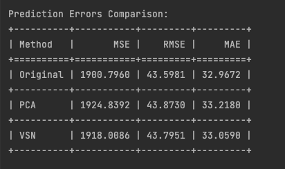
The same efficiency of the TiDE mannequin throughout each authentic and lowered characteristic units reveals a vital perception: characteristic discount didn’t result in improved predictions as one would possibly count on. This means potential key points:

• Info loss: regardless of aiming to protect important knowledge, dimensionality discount strategies discarded data related to the prediction activity, explaining the shortage of enchancment with fewer options.
• Generalization struggles: constant efficiency throughout characteristic units signifies the mannequin’s issue in capturing underlying patterns, no matter characteristic depend.
• Complexity overkill: related outcomes with fewer options counsel TiDE’s subtle structure could also be unnecessarily complicated. A less complicated mannequin, like ARIMA, might probably carry out simply as properly.

Then, let’s look at the chart to see if we will observe any important variations among the many three forecasting strategies and the precise costs.

import matplotlib.pyplot as plt

plt.determine(figsize=(12, 6))
plt.plot(train_data['ds'], train_data['price'], label='Coaching Knowledge', coloration='blue')
plt.plot(test_data['ds'], true_values, label='True Costs', coloration='inexperienced')
plt.plot(test_data['ds'], predicted_prices_original, label='Predicted Costs', coloration='crimson')
plt.legend()
plt.title('SPY Worth Forecast Utilizing All Authentic Characteristic')
plt.xlabel('Date')
plt.ylabel('SPY Worth')
plt.savefig('spy_forecast_chart_original.png', dpi=300, bbox_inches='tight')
plt.shut()

plt.determine(figsize=(12, 6))
plt.plot(train_data['ds'], train_data['price'], label='Coaching Knowledge', coloration='blue')
plt.plot(test_data['ds'], true_values, label='True Costs', coloration='inexperienced')
plt.plot(test_data['ds'], predicted_prices_pca, label='Predicted Costs', coloration='crimson')
plt.legend()
plt.title('SPY Worth Forecast Utilizing PCA Dimensionality Discount')
plt.xlabel('Date')
plt.ylabel('SPY Worth')
plt.savefig('spy_forecast_chart_pca.png', dpi=300, bbox_inches='tight')
plt.shut()

plt.determine(figsize=(12, 6))
plt.plot(train_data['ds'], train_data['price'], label='Coaching Knowledge', coloration='blue')
plt.plot(test_data['ds'], true_values, label='True Costs', coloration='inexperienced')
plt.plot(test_data['ds'], predicted_prices_vsn, label='Predicted Costs', coloration='crimson')
plt.legend()
plt.title('SPY Worth Forecast Utilizing VSN')
plt.xlabel('Date')
plt.ylabel('SPY Worth')
plt.savefig('spy_forecast_chart_vsn.png', dpi=300, bbox_inches='tight')
plt.shut()

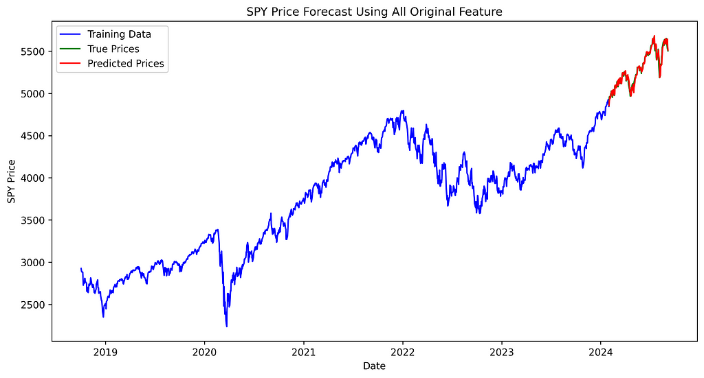
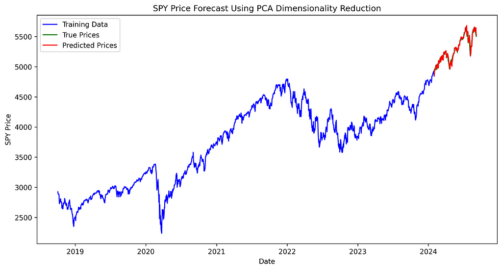
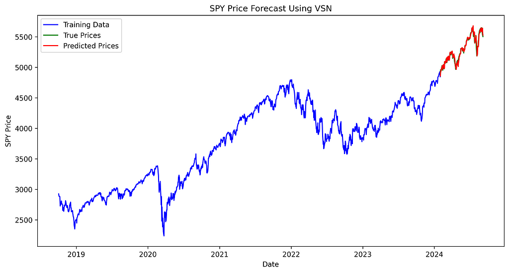
The distinction between true and predicted costs seems constant throughout all three fashions, with no noticeable variation in efficiency between them.

Conclusion

We did it! We explored the significance of characteristic discount in time sequence evaluation and offered a sensible implementation information:

• Characteristic discount goals to simplify fashions whereas sustaining predictive energy. Advantages embody lowered complexity, improved generalization, simpler interpretation, and computational effectivity.
• We demonstrated two discount strategies utilizing FRED knowledge:

1. Principal Element Evaluation (PCA), a linear dimensionality discount technique, lowered options from 438 to 76 whereas retaining 90% of defined variance.
2. Variable Choice Community (VSN) from the Temporal Fusion Transformers, a non-linear method, drastically lowered options to simply 1 utilizing an eightieth percentile significance threshold.

• Analysis utilizing TiDE fashions confirmed related efficiency throughout authentic and lowered characteristic units, suggesting characteristic discount might not all the time enhance forecasting efficiency. This might be because of data loss throughout discount, the mannequin’s issue in capturing underlying patterns, or the chance {that a} less complicated mannequin is likely to be equally efficient for this explicit forecasting activity.

On a remaining be aware, we didn’t discover all characteristic discount strategies, equivalent to SHAP (SHapley Additive exPlanations), which offers a unified measure of characteristic significance throughout numerous mannequin sorts. Even when we didn’t enhance our mannequin, it’s nonetheless higher to carry out characteristic curation and evaluate efficiency throughout completely different discount strategies. This method helps make sure you’re not discarding helpful data whereas optimizing your mannequin’s effectivity and interpretability.

In future articles, we’ll apply these characteristic discount strategies to extra complicated fashions, evaluating their influence on efficiency and interpretability. Keep tuned!

Able to put these ideas into motion? You’ll find the whole code implementation right here.

Appreciated this text? Present your assist!

👏 Clap it as much as 50 occasions

🤝 Ship me a LinkedIn connection request to remain in contact

Your assist means every part! 🙏

---

Is Much less Extra? Do Deep Studying Forecasting Fashions Want Characteristic Discount? was initially printed in In the direction of Knowledge Science on Medium, the place persons are persevering with the dialog by highlighting and responding to this story.