


")


 is Bullish As lengthy Because it Stays Above This Crucial Resistance Stage: Analyst")


")


A brand new technique for decomposing your favourite efficiency metrics
Co-authored with S. Hué, C. Hurlin, and C. Pérignon.
I – From explaining mannequin forecasts to explaining mannequin efficiency
Trustability and acceptability of delicate AI methods largely rely on the capability of the customers to grasp the related fashions, or a minimum of their forecasts. To carry the veil on opaque AI functions, eXplainable AI (XAI) strategies equivalent to post-hoc interpretability instruments (e.g. SHAP, LIME), are generally utilized at present, and the insights generated from their outputs are actually broadly comprehended.
Past particular person forecasts, we present on this article the best way to determine the drivers of the efficiency metrics (e.g. AUC, R2) of any classification or regression mannequin utilizing the eXplainable PERformance (XPER) methodology. With the ability to determine the driving forces of the statistical or financial efficiency of a predictive mannequin lies on the very core of modeling and is of nice significance for each knowledge scientists and consultants basing their choices on such fashions. The XPER library outlined beneath has confirmed to be an environment friendly device to decompose efficiency metrics into particular person function contributions.
Whereas they’re grounded in the identical mathematical ideas, XPER and SHAP are essentially completely different and easily have completely different targets. Whereas SHAP pinpoints the options that considerably affect the mannequin’s particular person predictions, XPER identifies the options that contribute probably the most to the efficiency of the mannequin. The latter evaluation may be carried out on the world (mannequin) degree or native (occasion) degree. In apply, the function with the strongest affect on particular person forecasts (say function A) will not be the one with the strongest affect on efficiency. Certainly, function A drives particular person choices when the mannequin is appropriate but additionally when the mannequin makes an error. Conceptually, if function A primarily impacts faulty predictions, it could rank decrease with XPER than it does with SHAP.
What’s a efficiency decomposition used for? First, it could improve any post-hoc interpretability evaluation by providing a extra complete perception into the mannequin’s interior workings. This permits for a deeper understanding of why the mannequin is, or shouldn’t be, performing successfully. Second, XPER may help determine and deal with heterogeneity issues. Certainly, by analyzing particular person XPER values, it’s doable to pinpoint subsamples during which the options have related results on efficiency. Then, one can estimate a separate mannequin for every subsample to spice up the predictive efficiency. Third, XPER may help to grasp the origin of overfitting. Certainly, XPER permits us to determine some options which contribute extra to the efficiency of the mannequin within the coaching pattern than within the take a look at pattern.
II – XPER values
The XPER framework is a theoretically grounded technique that’s based mostly on Shapley values (Shapley, 1953), a decomposition technique from coalitional recreation idea. Whereas the Shapley values decompose a payoff amongst gamers in a recreation, XPER values decompose a efficiency metric (e.g., AUC, R2) amongst options in a mannequin.
Suppose that we practice a classification mannequin utilizing three options and that its predictive efficiency is measured with an AUC equal to 0.78. An instance of XPER decomposition is the next:
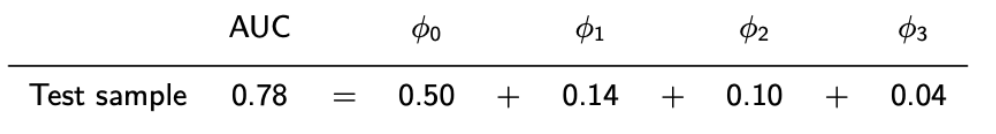
The primary XPER worth 𝜙₀ is known as the benchmark and represents the efficiency of the mannequin if not one of the three options offered any related data to foretell the goal variable. When the AUC is used to judge the predictive efficiency of a mannequin, the worth of the benchmark corresponds to a random classification. Because the AUC of the mannequin is bigger than 0.50, it implies that a minimum of one function comprises helpful data to foretell the goal variable. The distinction between the AUC of the mannequin and the benchmark represents the contribution of options to the efficiency of the mannequin, which may be decomposed with XPER values. On this instance, the decomposition signifies that the primary function is the primary driver of the predictive efficiency of the mannequin because it explains half of the distinction between the AUC of the mannequin and a random classification (𝜙₁), adopted by the second function (𝜙₂) and the third one (𝜙₃). These outcomes thus measure the worldwide impact of every function on the predictive efficiency of the mannequin and to rank them from the least necessary (the third function) to crucial (the primary function).
Whereas the XPER framework can be utilized to conduct a worldwide evaluation of the mannequin predictive efficiency, it will also be used to supply an area evaluation on the occasion degree. On the native degree, the XPER worth corresponds to the contribution of a given occasion and have to the predictive efficiency of the mannequin. The benchmark then represents the contribution of a given statement to the predictive efficiency if the goal variable was unbiased from the options, and the distinction between the person contribution and the benchmark is defined by particular person XPER values. Due to this fact, particular person XPER values enable us to grasp why some observations contribute extra to the predictive efficiency of a mannequin than others, and can be utilized to deal with heterogeneity points by figuring out teams of people for which options have related results on efficiency.
Additionally it is necessary to notice that XPER is each mannequin and metric-agnostic. It implies that XPER values can be utilized to interpret the predictive efficiency of any econometric or machine studying mannequin, and to interrupt down any efficiency metric, equivalent to predictive accuracy measures (AUC, accuracy), statistical loss features (MSE, MAE), or financial efficiency measure (profit-and-loss features).
III – XPER in Python
01 — Obtain Library ⚙️
The XPER strategy is carried out in Python by means of the XPER library. To compute XPER values, first one has to put in the XPER library as follows:
pip set up XPER
02 — Import Library 📦
import XPER
import pandas as pd
03 — Load instance dataset 💽
For example the best way to use XPER values in Python, allow us to take a concrete instance. Contemplate a classification downside whose fundamental goal is to foretell credit score default. The dataset may be immediately imported from the XPER library such as:
import XPER
from XPER.datasets.load_data import loan_status
mortgage = loan_status().iloc[:, :6]

show(mortgage.head())
show(mortgage.form)
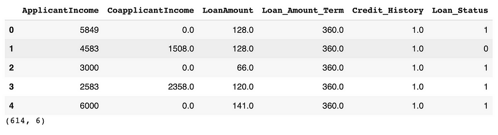
The first aim of this dataset, given the included variables, seems to be constructing a predictive mannequin to find out the “Loan_Status” of a possible borrower. In different phrases, we wish to predict whether or not a mortgage software will probably be authorized (“1”) or not (“0”) based mostly on the knowledge offered by the applicant.
# Take away 'Loan_Status' column from 'mortgage' dataframe and assign it to 'X'
X = mortgage.drop(columns='Loan_Status')

# Create a brand new dataframe 'Y' containing solely the 'Loan_Status' column from 'mortgage' dataframe
Y = pd.Collection(mortgage['Loan_Status'])
04 — Estimate the Mannequin ⚙️
Then, we have to practice a predictive mannequin and to measure its efficiency with the intention to compute the related XPER values. For illustration functions, we cut up the preliminary dataset right into a coaching and a take a look at set and match a XGBoost classifier on the coaching set:
from sklearn.model_selection import train_test_split

# Break up the info into coaching and testing units
# X: enter options
# Y: goal variable
# test_size: the proportion of the dataset to incorporate within the testing set (on this case, 15%)
# random_state: the seed worth utilized by the random quantity generator for reproducible outcomes
X_train, X_test, y_train, y_test = train_test_split(X, Y, test_size=0.15, random_state=3)

import xgboost as xgb

# Create an XGBoost classifier object
gridXGBOOST = xgb.XGBClassifier(eval_metric="error")

# Practice the XGBoost classifier on the coaching knowledge
mannequin = gridXGBOOST.match(X_train, y_train)
05 — Consider Efficiency 🎯
The XPER library presents an intuitive and easy method to compute the predictive efficiency of a predictive mannequin. Contemplating that the efficiency metric of curiosity is the Areas Below the ROC Curve (AUC), it may be measured on the take a look at set as follows:
from XPER.compute.Efficiency import ModelPerformance

# Outline the analysis metric(s) for use
XPER = ModelPerformance(X_train.values,
                        y_train.values,
                        X_test.values,
                        y_test.values,
                        mannequin)

# Consider the mannequin efficiency utilizing the desired metric(s)
PM = XPER.consider(["AUC"])

# Print the efficiency metrics
print("Efficiency Metrics: ", spherical(PM, 3))
06 — Calculate XPER values ⭐️
Lastly, to clarify the driving forces of the AUC the XPER values may be computed such as:
# Calculate XPER values for the mannequin's efficiency
XPER_values = XPER.calculate_XPER_values(["AUC"],kernel=False)
The « XPER_values » is a tuple together with two parts: the XPER values and the person XPER values of the options.
To be used circumstances above 10 function variables it’s suggested to used the default choice kernel=True for computation effectivity ➡️
07 — Visualization 📊
from XPER.viz.Visualisation import visualizationClass as viz

labels = listing(mortgage.drop(columns='Loan_Status').columns)
To research the driving drive on the world degree, the XPER library proposes a bar plot illustration of XPER values.
viz.bar_plot(XPER_values=XPER_values, X_test=X_test, labels=labels, p=5,share=True)
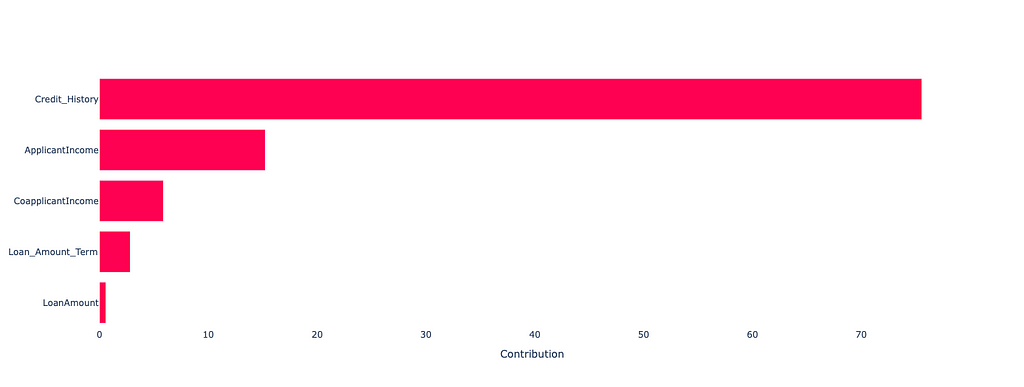
For ease of presentation, function contributions are expressed in share of the unfold between the AUC and its benchmark, i.e., 0.5 for the AUC, and are ordered from the biggest to lowest. From this determine, we will see that greater than 78% of the over-performance of the mannequin over a random predictor comes from Credit score Historical past, adopted by Applicant Earnings contributing round 16% to the efficiency, and Co-applicant Earnings and Mortgage Quantity Time period every accounting for lower than 6%. Then again, we will see that the variable Mortgage Quantity virtually doesn’t assist the mannequin to raised predict the chance of default as its contribution is near 0.
The XPER library additionally proposes graphical representations to research XPER values on the native degree. First, a drive plot can be utilized to research driving forces of the efficiency for a given statement:
viz.force_plot(XPER_values=XPER_values, occasion=1, X_test=X_test, variable_name=labels, figsize=(16,4))
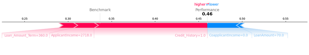
The previous code plots the constructive (unfavorable) XPER values of the statement #10 in purple (blue), in addition to the benchmark (0.33) and contribution (0.46) of this statement to the AUC of the mannequin. The over-performance of borrower #10 is as a result of constructive XPER values of Mortgage Quantity Time period, Applicant Earnings, and Credit score Historical past. Then again, Co-Applicant Earnings and Mortgage Quantity had a unfavorable impact and decreased the contribution of this borrower.
We will see that whereas Applicant Earnings and Mortgage Quantity have a constructive impact on the AUC on the world degree, these variables have a unfavorable impact for the borrower #10. Evaluation of particular person XPER values can thus determine teams of observations for which options have completely different results on efficiency, doubtlessly highlighting an heterogeneity challenge.
Second, it’s doable to characterize the XPER values of every statement and have on a single plot. For that objective, one can depend on a beeswarm plot which represents the XPER values for every function as a perform of the function worth.
viz.beeswarn_plot(XPER_values=XPER_values,X_test=X_test,labels=labels)
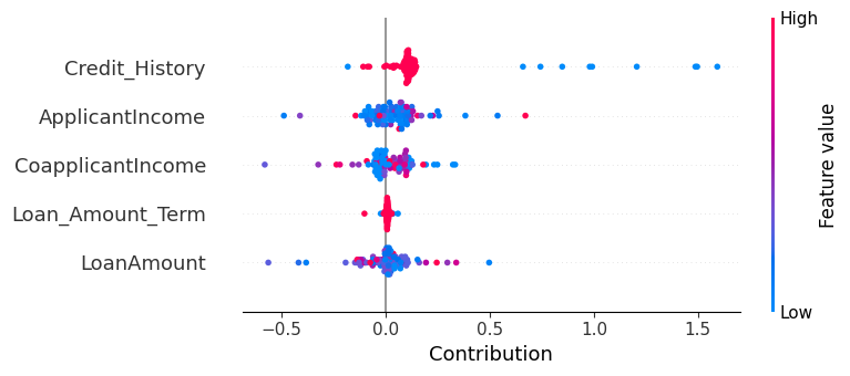
On this determine, every dot represents an statement. The horizontal axis represents the contribution of every statement to the efficiency of the mannequin, whereas the vertical axis represents the magnitude of function values. Equally to the bar plot proven beforehand, options are ordered from those who contribute probably the most to the efficiency of the mannequin to people who contribute the least. Nevertheless, with the beeswarm plot it is usually doable to research the impact of function values on XPER values. On this instance, we will see massive values of Credit score Historical past are related to comparatively small contributions (in absolute worth), whereas low values result in bigger contributions (in absolute worth).
All photos, except in any other case acknowledged, are by the writer.
IV – Acknowledgements
The contributors to this library are:
V – References
[1] L. Shapley, A Worth for n-Individual Video games (1953), Contributions to the Principle of Video games, 2:307–317
[2] S. Lundberg, S. Lee, A unified strategy to decoding mannequin predictions (2017), Advances in Neural Data Processing Techniques
[3] S. Hué, C. Hurlin, C. Pérignon, S. Saurin, Measuring the Driving Forces of Predictive Efficiency: Utility to Credit score Scoring (2023), HEC Paris Analysis Paper No. FIN-2022–1463
XPER: Unveiling the Driving Forces of Predictive Efficiency was initially revealed in In direction of Knowledge Science on Medium, the place persons are persevering with the dialog by highlighting and responding to this story.