Visualising Strava Race Evaluation

Two New Graphs That Evaluate Runners on the Identical Occasion

Have you ever ever questioned how two runners stack up in opposition to one another in the identical race?

On this article I current two new graphs that I’ve designed, as I felt they had been lacking from Strava. These graphs have been created in a manner that they will inform the story of a race at a look as they examine totally different athletes operating the identical occasion. One can simply see adjustments in positions, in addition to the time distinction throughout the laps and opponents.

My rationalization will begin with how I noticed the chance. Subsequent, I’ll showcase the graph designs and clarify the algorithms and knowledge processing methods that energy them.

Strava doesn’t inform the total story

Strava is a social health app had been folks can file and share their sport actions with a group of 100+ million customers [1]. Extensively used amongst cyclists and runners, it’s an amazing software that not solely data your actions, but additionally gives personalised evaluation about your efficiency based mostly in your health knowledge.

As a runner, I discover this app extremely useful for 2 foremost causes:

1. It gives knowledge evaluation that assist me perceive my operating efficiency higher.
2. It pushes me to remain motivated as I can see what my associates and the group are sharing.

Each time I full a operating occasion with my associates, all of us log our health knowledge from our watches into Strava to see evaluation such as:

• Whole time, distance and common tempo.
• Time for each break up or lap within the race.
• Coronary heart Fee metrics evolution.
• Relative Effort in comparison with earlier actions.

The very best half is after we speak in regards to the race from everybody’s views. Strava is ready to recognise that you just ran the identical occasion with your folks (in case you observe one another) and even different folks, nevertheless it doesn’t present comparative knowledge. So if you wish to have the total story of the race with your folks, it’s worthwhile to dive into everybody’s exercise and attempt to examine them.

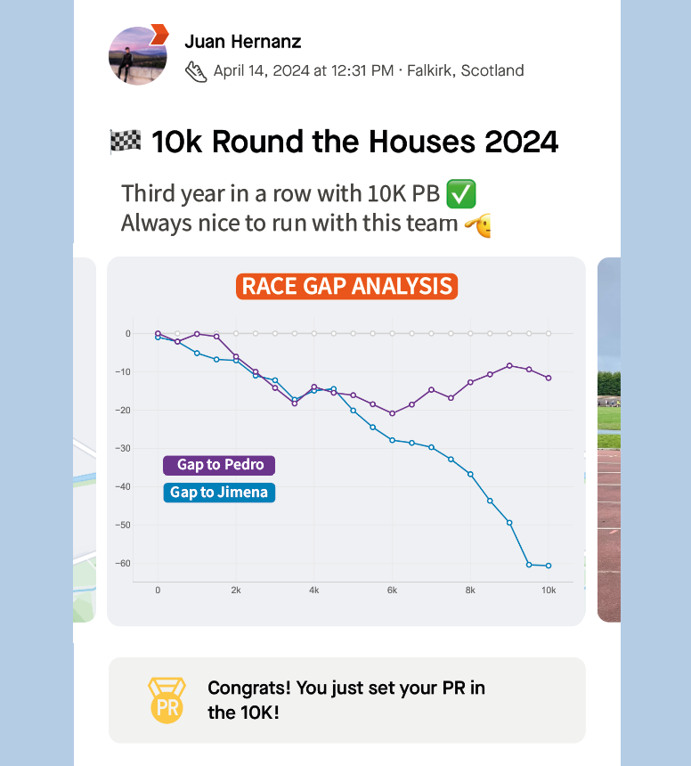
That’s why, after my final 10K with 3 associates this yr, I made a decision to get the information from Strava and design two visuals to see a comparative evaluation of our race efficiency.

Presenting the visuals

The thought behind this venture is straightforward: use GPX knowledge from Strava (location, timestamp) recorded by my associates and me throughout a race and mix them to generate visuals evaluating our races.

The problem was not solely validating that my concept was doable, but additionally designing Strava-inspired graphs to proof how they may seamlessly combine as new options within the present utility. Let’s see the outcomes.

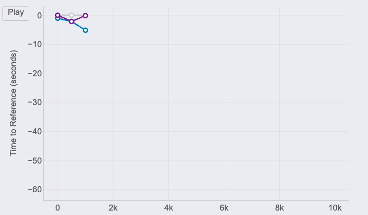
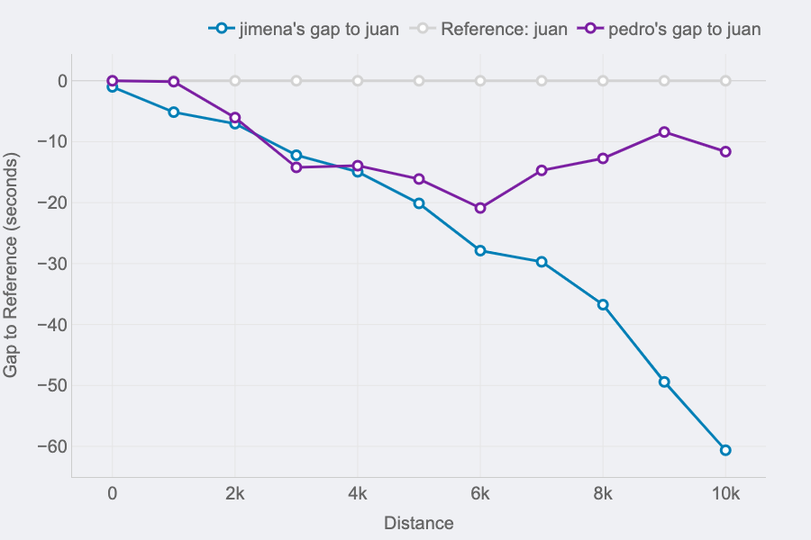
Race GAP Evaluation

Metrics: the evolution of the hole (in seconds) between a runner that’s the reference (gray line on 0) and their opponents. Strains above imply the runner is forward on the race.

Insights: this line chart is ideal to see the adjustments in positions and distances for a bunch of runners.

For those who take a look at the best finish of the traces, you’ll be able to see the ultimate outcomes of the race for the three runners of our examples:

1. The primary runner (me) is represented by the reference in gray.
2. Pedro (in purple) was the second runner reaching the end line solely 12 seconds after.
3. Jimena (in blue) completed the 10K 60 seconds after.

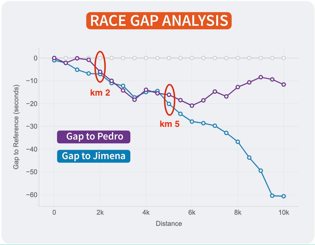
However, due to this chart, it’s doable to see how theses gaps the place altering all through the race. And these insights are actually fascinating to know the race positions and distances:

1. The three of us began the race collectively. Jimena, in blue, began to fall behind round 5 seconds within the first km whereas me (gray) and Pedro ( purple) the place collectively.
2. I bear in mind Pedro telling me it was too quick of a begin, so he barely lowered the tempo till he discovered Jimena at km 2. Their traces present they ran collectively till the fifth km, whereas I used to be rising the hole with them.
3. Km 6 is essential, my hole with Pedro at that time was 20 seconds (the max I reached) and virtually 30 seconds to Jimena, who lowered the tempo in comparison with mine till the tip of the race. Nevertheless, Pedro began going quicker and lowered our hole pushing quicker within the 4 final kms.

After all, the traces will change relying on who’s the reference. This manner, each runner will see the story of the identical race however personalised to their viewpoint and the way the examine to the remainder. It’s the identical story with totally different foremost characters.

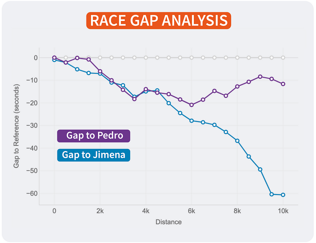
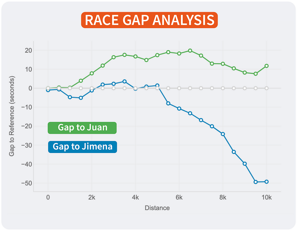
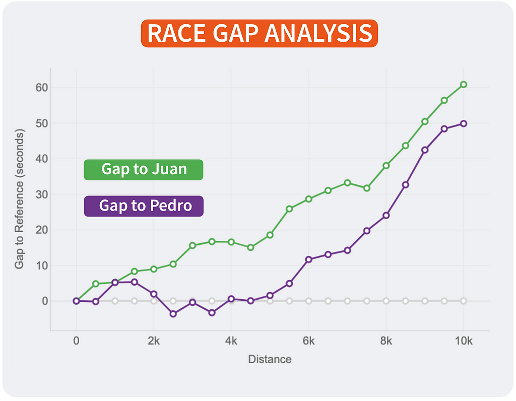
If I had been Strava, I would come with this chart within the actions marked as RACE by the consumer. The evaluation may very well be achieved with all of the followers of that consumer that registered the identical exercise. An instance of integration is proven above.

Head-to-Head Lap Evaluation

Metrics: the road signify the evolution of the hole (in seconds) between two runners. The bars signify, for each lap, if a runner was quicker (blue) or slower (purple) in comparison with different.

Insights: this mixed chart is good for analysing the head-to-head efficiency throughout each lap of a race.

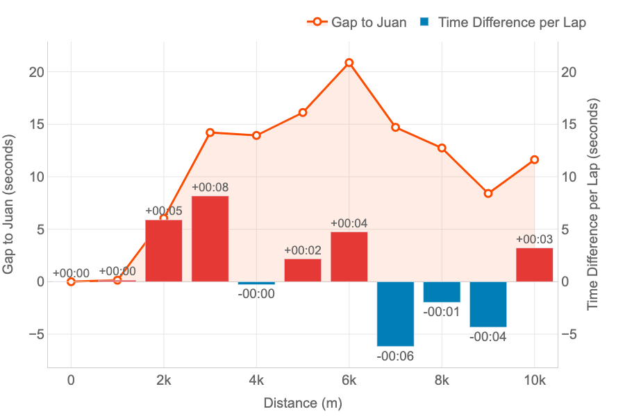
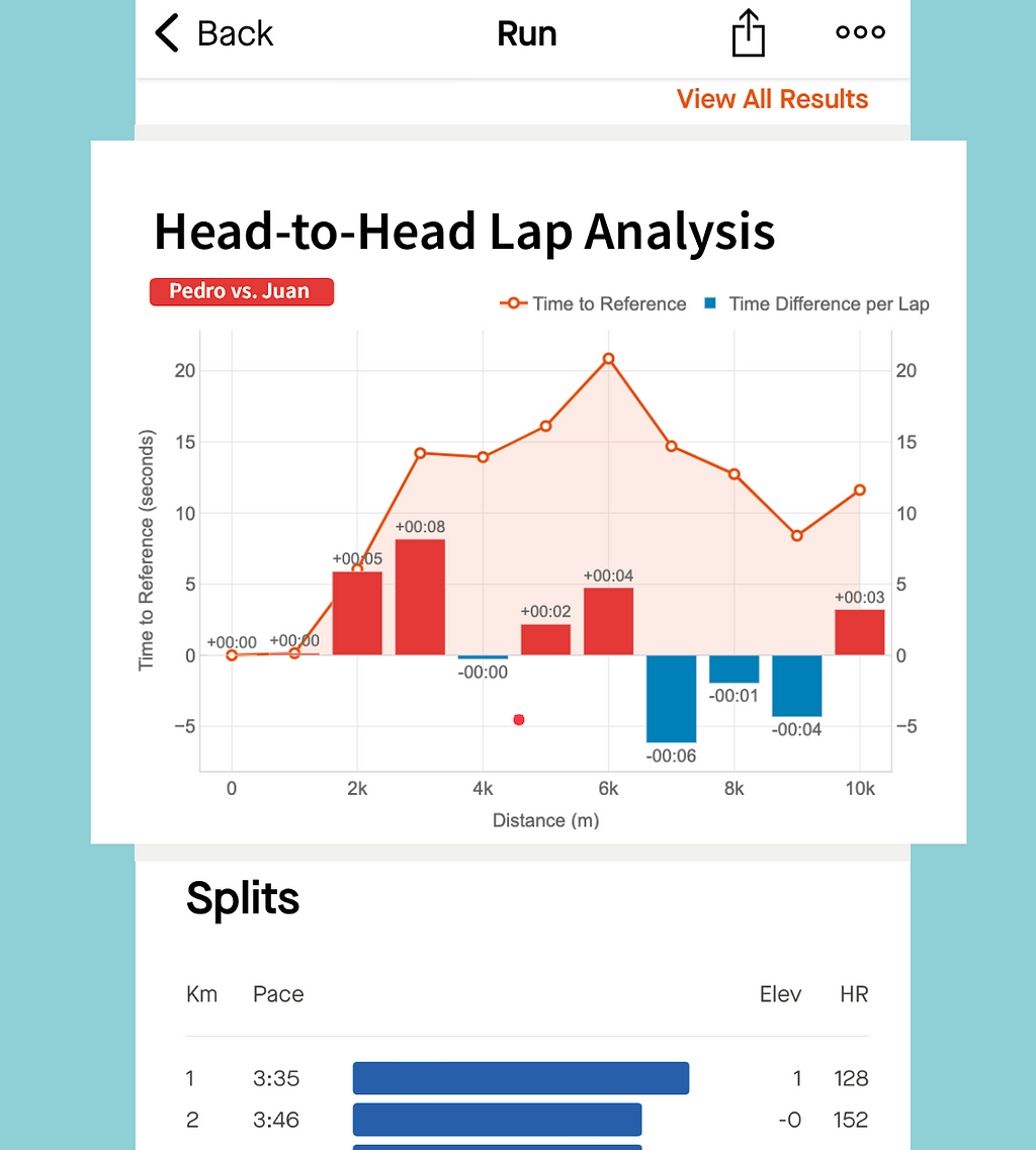
This graph has been particularly designed to check two runners efficiency throughout the splits (laps) of the race.

The instance signify the time lack of Pedro in comparison with Juan.

• The orange line signify the loss in time as defined for the opposite graph: each began collectively, however Pedro began to lose time after the primary km till the sixth. Then, he started to be quicker to cut back that hole.
• The bars carry new insights to our comparability representing the time loss (in purple) or the acquire (in blue) for each lap. At a look, Pedro can see that the larger loss in time was on the third km (8 seconds). And he solely misplaced time on half of the splits. The tempo of each was the identical for kilometres 1 and 4, and Pedro was quicker between on the kms 7, 8 and 9.

Due to this graph we are able to see that I used to be quicker than Pedro on the primary 6 kms, gaining and benefit that Pedro couldn’t cut back, regardless of being quicker on the final a part of the race. And this confirms the sensation that now we have after the competitions: “Pedro has stronger finishes in races.”

Knowledge Processing and Algorithms

If you wish to know the way the graphs had been created, preserve studying this part in regards to the implementation.

I don’t wish to go an excessive amount of into the coding bits behind this. As each software program downside, you may obtain your objective by way of totally different options. That’s why I’m extra fascinated by explaining the issues that I confronted and the logic behind my options.

Loading Knowledge

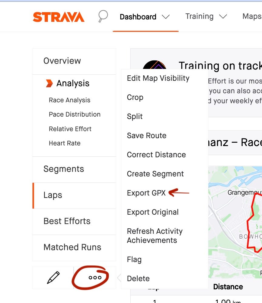
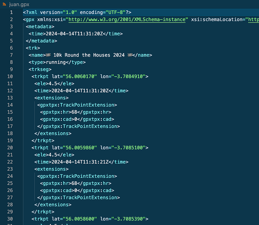
No knowledge, no resolution. On this case no Strava API is required . For those who log in your Strava account and go to an exercise you’ll be able to obtain the GPX file of the exercise by clicking on Export GPX as proven on the screenshot. GPX recordsdata include datapoints in XML format as seen beneath.

To get my associates knowledge for a similar actions I simply advised them to observe the identical steps and ship the .gpx recordsdata to me.

Getting ready Knowledge

For this use case I used to be solely fascinated by a number of attributes:

• Location: latitude, longitude and elevation
• Timestamp: time.

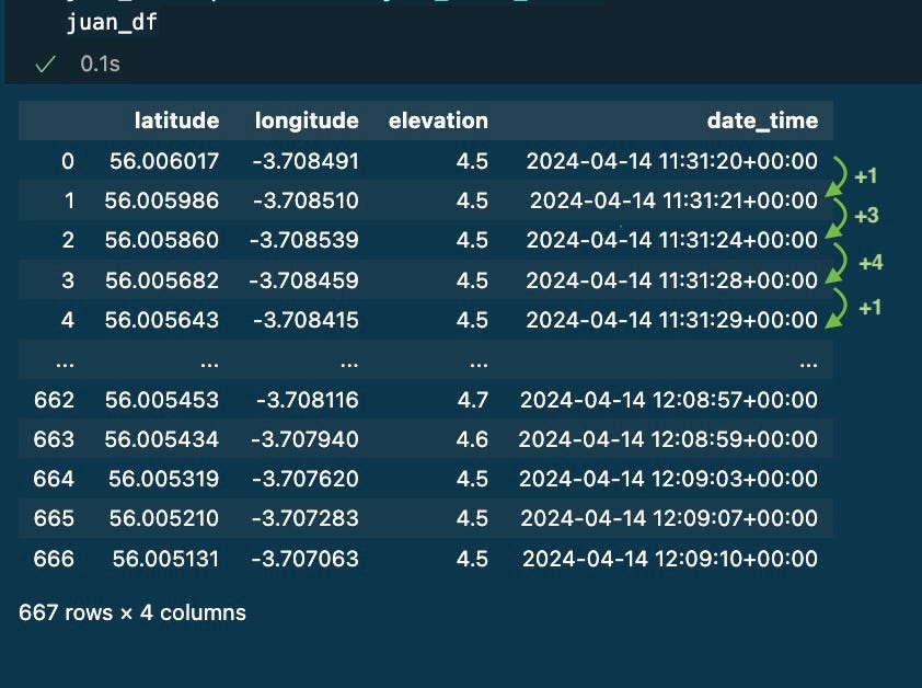
First downside for me was to transform the .gpx recordsdata into pandas dataframes so I can play and course of the information utilizing python. I used gpxpy library. Code beneath

import pandas as pd
import gpxpy

# learn file
with open('juan.gpx', 'r') as gpx_file:
    juan_gpx = gpxpy.parse(gpx_file)

# Convert Juan´s gpx to dataframe
juan_route_info = []

for monitor in juan_gpx.tracks:
    for phase in monitor.segments:
        for level in phase.factors:
            juan_route_info.append({
                'latitude': level.latitude,
                'longitude': level.longitude,
                'elevation': level.elevation,
                'date_time': level.time
            })

juan_df =  pd.DataFrame(juan_route_info)
juan_df

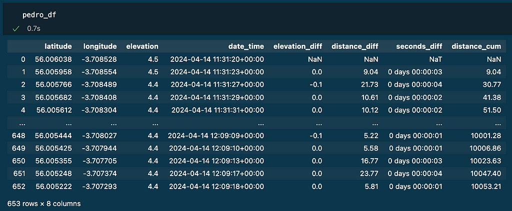
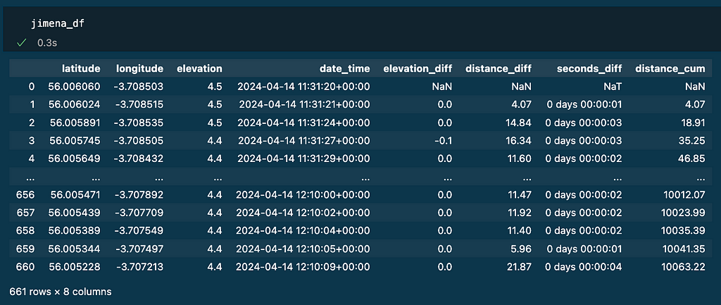
After that, I had 667 datapoints saved on a dataframe. Each row represents the place and when I used to be in the course of the exercise.

I learnt that not each row is captured with the identical frequency (1 second between 0 and 1, then 3 seconds, then 4 seconds, then 1 second…)

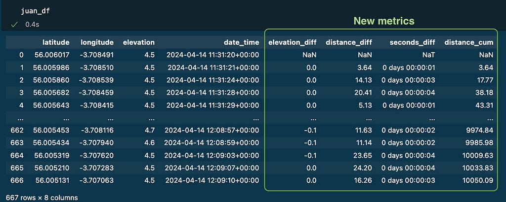
Getting some metrics

Each row within the knowledge represents a distinct second and place, so my first concept was to calculate the distinction in time, elevation, and distance between two consecutive rows: seconds_diff, elevation_diff and distance_diff.

Time and elevation had been simple utilizing .diff() technique over every column of the pandas dataframe.

# First Calculate elevation diff
juan_df['elevation_diff'] = juan_df['elevation'].diff()

# Calculate the distinction in seconds between datapoints
juan_df['seconds_diff'] = juan_df['date_time'].diff()

Sadly, because the Earth is just not flat, we have to use a distance metric referred to as haversine distance [2]: the shortest distance between two factors on the floor of a sphere, given their latitude and longitude coordinates. I used the library haversine. See the code beneath

import haversine as hs

# Perform to calculate haversine distances
def haversine_distance(lat1, lon1, lat2, lon2) -> float:
    distance = hs.haversine(
        point1=(lat1, lon1),
        point2=(lat2, lon2),
        unit=hs.Unit.METERS
    )

    # Returns the space between the primary level and the second level
    return np.spherical(distance, 2)

#calculate the distances between all knowledge factors
distances = [np.nan]

for i in vary(len(track_df)):
    if i == 0:
        proceed
    else:
        distances.append(haversine_distance(
            lat1=juan_df.iloc[i - 1]['latitude'],
            lon1=juan_df.iloc[i - 1]['longitude'],
            lat2=juan_df.iloc[i]['latitude'],
            lon2=juan_df.iloc[i]['longitude']
        ))
        
juan_df['distance_diff'] = distances

The cumulative distance was additionally added as a brand new column distance_cum utilizing the tactic cumsum() as seen beneath

# Calculate the cumulative sum of the space
juan_df['distance_cum'] = juan_df['distance_diff'].cumsum()

At this level the dataframe with my monitor knowledge contains 4 new columns with helpful metrics:

I utilized the identical logic to different runners’ tracks: jimena_df and pedro_df.

We’re prepared now to play with the information to create the visualisations.

Challenges:

To acquire the information wanted for the visuals my first instinct was: take a look at the cumulative distance column for each runner, determine when a lap distance was accomplished (1000, 2000, 3000, and so on.) by every of them and do the variations of timestamps.

That algorithm appears easy, and may work, but it surely had some limitations that I wanted to handle:

1. Precise lap distances are sometimes accomplished in between two knowledge factors registered. To be extra correct I needed to do interpolation of each place and time.
2. As a consequence of distinction within the precision of gadgets, there could be misalignments throughout runners. The commonest is when a runner’s lap notification beeps earlier than one other one even when they’ve been collectively the entire monitor. To minimise this I made a decision to use the reference runner to set the place marks for each lap within the monitor. The time distinction can be calculated when different runners cross these marks (despite the fact that their cumulative distance is forward or behind the lap). That is extra near the truth of the race: if somebody crosses some extent earlier than, they’re forward (regardless the cumulative distance of their machine)
3. With the earlier level comes one other downside: the latitude and longitude of a reference mark may by no means be precisely registered on the opposite runners’ knowledge. I used Nearest Neighbours to seek out the closest datapoint by way of place.
4. Lastly, Nearest Neighbours may carry fallacious datapoints if the monitor crosses the identical positions at totally different moments in time. So the inhabitants the place the Nearest Neighbours will search for the very best match must be lowered to a smaller group of candidates. I outlined a window dimension of 20 datapoints across the goal distance (distance_cum).

Algorithm

With all of the earlier limitations in thoughts, the algorithm needs to be as follows:

1. Select the reference and a lap distance (default= 1km)

2. Utilizing the reference knowledge, determine the place and the second each lap was accomplished: the reference marks.

3. Go to different runner’s knowledge and determine the moments they crossed these place marks. Then calculate the distinction in time of each runners crossing the marks. Lastly the delta of this time distinction to signify the evolution of the hole.

Code Instance

1. Select the reference and a lap distance (default= 1km)

• Juan would be the reference (juan_df) on the examples.
• The opposite runners can be Pedro (pedro_df ) and Jimena (jimena_df).
• Lap distance can be 1000 metres

2. Create interpolate_laps(): perform that finds or interpolates the precise level for every accomplished lap and return it in a brand new dataframe. The inferpolation is finished with the perform: interpolate_value() that was additionally created.

## Perform: interpolate_value()

Enter: 
    - begin: The beginning worth.
    - finish: The ending worth.
    - fraction: A worth between 0 and 1 that represents the place between 
      the beginning and finish values the place the interpolation ought to happen.
Return:
    - The interpolated worth that lies between the begin and finish values 
      on the specified fraction.

def interpolate_value(begin, finish, fraction):
    return begin + (finish - begin) * fraction

## Perform: interpolate_laps()

Enter: 
    - track_df: dataframe with monitor knowledge.
    - lap_distance: metres per lap (default 1000)
Return:
    - track_laps: dataframe with lap metrics. As many rows as laps recognized.

def interpolate_laps(track_df , lap_distance = 1000):
  #### 1. Initialise track_laps with the primary row of track_df 
  track_laps = track_df.loc[0][['latitude','longitude','elevation','date_time','distance_cum']].copy()
  
  # Set distance_cum = 0
  track_laps[['distance_cum']] = 0

  # Transpose dataframe
  track_laps = pd.DataFrame(track_laps)
  track_laps = track_laps.transpose()

  #### 2. Calculate number_of_laps = Whole Distance / lap_distance
  number_of_laps = track_df['distance_cum'].max()//lap_distance

  #### 3. For every lap i from 1 to number_of_laps:
  for i in vary(1,int(number_of_laps+1),1):

    # a. Calculate target_distance = i * lap_distance
    target_distance = i*lap_distance

    # b. Discover first_crossing_index the place track_df['distance_cum'] > target_distance
    first_crossing_index = (track_df['distance_cum'] > target_distance).idxmax()
    
    # c. If match is strictly the lap distance, copy that row
    if (track_df.loc[first_crossing_index]['distance_cum'] == target_distance):
      new_row = track_df.loc[first_crossing_index][['latitude','longitude','elevation','date_time','distance_cum']]
       
    # Else: Create new_row with interpolated values, copy that row.
    else: 

      fraction = (target_distance - track_df.loc[first_crossing_index-1, 'distance_cum']) / (track_df.loc[first_crossing_index, 'distance_cum'] - track_df.loc[first_crossing_index-1, 'distance_cum'])

      # Create the brand new row
      new_row = pd.Collection({
          'latitude': interpolate_value(track_df.loc[first_crossing_index-1, 'latitude'], track_df.loc[first_crossing_index, 'latitude'], fraction),
          'longitude': interpolate_value(track_df.loc[first_crossing_index-1, 'longitude'], track_df.loc[first_crossing_index, 'longitude'], fraction),
          'elevation': interpolate_value(track_df.loc[first_crossing_index-1, 'elevation'], track_df.loc[first_crossing_index, 'elevation'], fraction),
          'date_time': track_df.loc[first_crossing_index-1, 'date_time'] + (track_df.loc[first_crossing_index, 'date_time'] - track_df.loc[first_crossing_index-1, 'date_time']) * fraction,
          'distance_cum': target_distance
      }, identify=f'lap_{i}')

    # d. Add the brand new row to the dataframe that shops the laps
    new_row_df = pd.DataFrame(new_row)
    new_row_df = new_row_df.transpose()

    track_laps = pd.concat([track_laps,new_row_df])

  #### 4. Convert date_time to datetime format and take away timezone
  track_laps['date_time'] = pd.to_datetime(track_laps['date_time'], format='%Y-%m-%d %H:%M:%S.%fpercentz')
  track_laps['date_time'] = track_laps['date_time'].dt.tz_localize(None)

  #### 5. Calculate seconds_diff between consecutive rows in track_laps
  track_laps['seconds_diff'] = track_laps['date_time'].diff()

  return track_laps

Making use of the interpolate perform to the reference dataframe will generate the next dataframe:

juan_laps = interpolate_laps(juan_df , lap_distance=1000)

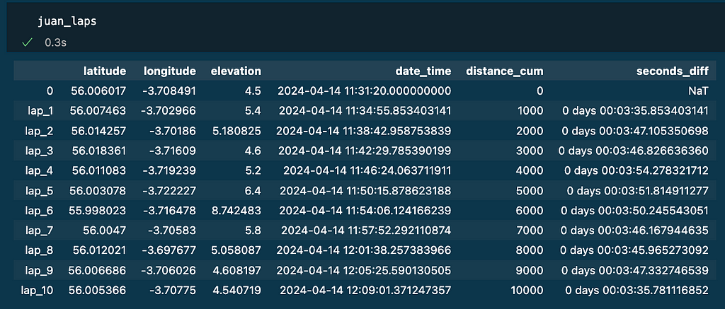
Word because it was a 10k race, 10 laps of 1000m has been recognized (see column distance_cum). The column seconds_diff has the time per lap. The remainder of the columns (latitude, longitude, elevation and date_time) mark the place and time for every lap of the reference as the results of interpolation.

3. To calculate the time gaps between the reference and the opposite runners I created the perform gap_to_reference()

## Helper Capabilities:
- get_seconds(): Convert timedelta to complete seconds
- format_timedelta(): Format timedelta as a string (e.g., "+01:23" or "-00:45")

# Convert timedelta to complete seconds
def get_seconds(td):
    # Convert to complete seconds
    total_seconds = td.total_seconds()    

    return total_seconds

# Format timedelta as a string (e.g., "+01:23" or "-00:45")
def format_timedelta(td):
    # Convert to complete seconds
    total_seconds = td.total_seconds()
    
    # Decide signal
    signal = '+' if total_seconds >= 0 else '-'
    
    # Take absolute worth for calculation
    total_seconds = abs(total_seconds)
    
    # Calculate minutes and remaining seconds
    minutes = int(total_seconds // 60)
    seconds = int(total_seconds % 60)
    
    # Format the string
    return f"{signal}{minutes:02d}:{seconds:02d}"

## Perform: gap_to_reference()

Enter: 
    - laps_dict: dictionary containing the df_laps for all of the runnners' names
    - df_dict: dictionary containing the track_df for all of the runnners' names
    - reference_name: identify of the reference
Return:
    - matches: processed knowledge with time variations.

def gap_to_reference(laps_dict, df_dict, reference_name):
  #### 1. Get the reference's lap knowledge from laps_dict
  matches = laps_dict[reference_name][['latitude','longitude','date_time','distance_cum']]

  #### 2. For every racer (identify) and their knowledge (df) in df_dict:
  for identify, df in df_dict.gadgets():

    # If racer is the reference: 
    if identify == reference_name:

      # Set time distinction to zero for all laps
      for lap, row  in matches.iterrows():
        matches.loc[lap,f'seconds_to_reference_{reference_name}'] = 0

    # If racer is just not the reference:
    if identify != reference_name:

      # a. For every lap discover the closest level in racer's knowledge based mostly on lat, lon.
      for lap, row  in matches.iterrows():
      
        # Step 1: set the place and lap distance from the reference
        target_coordinates = matches.loc[lap][['latitude', 'longitude']].values
        target_distance = matches.loc[lap]['distance_cum']
        
        
        # Step 2: discover the datapoint that can be within the centre of the window
        first_crossing_index = (df_dict[name]['distance_cum'] > target_distance).idxmax()
        
        # Step 3: choose the 20 candidate datapoints to search for the match
        window_size = 20
        window_sample = df_dict[name].loc[first_crossing_index-(window_size//2):first_crossing_index+(window_size//2)]
        candidates = window_sample[['latitude', 'longitude']].values

        # Step 4: get the closest match utilizing the coordinates
        nn = NearestNeighbors(n_neighbors=1, metric='euclidean')
        nn.match(candidates)
        distance, indice = nn.kneighbors([target_coordinates])

        nearest_timestamp = window_sample.iloc[indice.flatten()]['date_time'].values
        nearest_distance_cum = window_sample.iloc[indice.flatten()]['distance_cum'].values
        euclidean_distance = distance

        matches.loc[lap,f'nearest_timestamp_{name}'] = nearest_timestamp[0]
        matches.loc[lap,f'nearest_distance_cum_{name}'] = nearest_distance_cum[0]
        matches.loc[lap,f'euclidean_distance_{name}'] = euclidean_distance
        
        
      # b. Calculate time distinction between racer and reference at this level
      matches[f'time_to_ref_{name}'] = matches[f'nearest_timestamp_{name}'] - matches['date_time']

      # c. Retailer time distinction and different related knowledge
      matches[f'time_to_ref_diff_{name}'] = matches[f'time_to_ref_{name}'].diff()
      matches[f'time_to_ref_diff_{name}'] = matches[f'time_to_ref_diff_{name}'].fillna(pd.Timedelta(seconds=0))
  
      # d. Format knowledge utilizing helper features
      matches[f'lap_difference_seconds_{name}'] = matches[f'time_to_ref_diff_{name}'].apply(get_seconds)
      matches[f'lap_difference_formatted_{name}'] = matches[f'time_to_ref_diff_{name}'].apply(format_timedelta)
          
      matches[f'seconds_to_reference_{name}'] = matches[f'time_to_ref_{name}'].apply(get_seconds)
      matches[f'time_to_reference_formatted_{name}'] = matches[f'time_to_ref_{name}'].apply(format_timedelta)

#### 3. Return processed knowledge with time variations
  return matches

Beneath the code to implement the logic and retailer outcomes on the dataframe matches_gap_to_reference:

# Lap distance
lap_distance = 1000

# Retailer the DataFrames in a dictionary
df_dict = {
    'jimena': jimena_df,
    'juan': juan_df,
    'pedro': pedro_df,
}

# Retailer the Lap DataFrames in a dictionary
laps_dict = {
    'jimena': interpolate_laps(jimena_df , lap_distance),
    'juan': interpolate_laps(juan_df , lap_distance),
    'pedro': interpolate_laps(pedro_df , lap_distance)
}

# Calculate gaps to reference
reference_name = 'juan'
matches_gap_to_reference  = gap_to_reference(laps_dict, df_dict, reference_name)

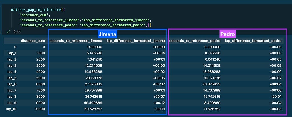
The columns of the ensuing dataframe include the necessary data that can be displayed on the graphs:

Race GAP Evaluation Graph

Necessities:

• The visualisation must be tailor-made for a runner who would be the reference. Each runner can be represented by a line graph.
• X-axis signify distance.
• Y-axis the hole to reference in seconds
• The reference will set the baseline. A relentless gray line in y-axis = 0
• The traces for the opposite runners can be above the reference in the event that they had been forward on the monitor and beneath in the event that they had been behind.

To signify the graph I used plotly library and used the information from matches_gap_to_reference:

X-axis: is the cumulative distance per lap. Column distance_cum

Y-axis: represents the hole to reference in seconds:

• Gray line: reference’s hole to reference is at all times 0.
• Purple line: Pedro’s hole to reference (-) seconds_to_reference_pedro.
• Blue line: Jimena’s hole to reference (-) seconds_to_reference_jimena.

Head to Head Lap Evaluation Graph

Necessities:

• The visualisation wants to check knowledge for under 2 runners. A reference and a competitor.
• X-axis represents distance
• Y-axis represents seconds
• Two metrics can be plotted to check the runners’ efficiency: a line graph will present the full hole for each level of the race. The bars will signify if that hole was elevated (constructive) or decreased (unfavorable) on each lap.

Once more, the information represented on the instance is coming from matches_gap_to_reference:

X-axis: is the cumulative distance per lap. Column distance_cum

Y-axis:

• Orange line: Pedro’s hole to Juan (+) seconds_to_reference_pedro
• Bars: the delta of that hole per lap lap_difference_formatted_pedro. If Pedro losses time, the delta is constructive and represented in purple. In any other case the bar is blue.

I refined the model of each visuals to align extra carefully with Strava’s design aesthetics.

Kudos for this article?

I began this concept after my final race. I actually preferred the outcomes of the visuals so I although they could be helpful for the Strava group. That’s why I made a decision to share them with the group scripting this article.

References

[1] S. Paul, Strava’s subsequent chapter: New CEO talks AI, inclusivity, and why ‘darkish mode’ took so lengthy. (2024)

[2] D. Grabiele, “Haversine Formulation”, Baeldung on Laptop Science. (2024)

---

Visualising Strava Race Evaluation was initially revealed in In the direction of Knowledge Science on Medium, the place persons are persevering with the dialog by highlighting and responding to this story.

Supply hyperlink