How Bend Works: A Parallel Programming Language That “Feels Like Python however Scales Like CUDA”

A quick introduction to Lambda Calculus, Interplay Combinators, and the way they’re used to parallelize operations on Bend / HVM.

Introduction

In case you are studying this text, you most likely lately heard about Bend, a brand new programming language that goals to be massively parallel however with out you worrying about issues like threads creation, and different widespread parallel programming phrases.

When you have no idea what I’m speaking about, watch the video beneath:

https://medium.com/media/e6219d3a2646a4b2a1562f430211ddd2/href

They declare “it looks like Python, however scales like CUDA”. As an fanatic of parallel programming, it caught my consideration instantly. After some studying, I discovered that Bend is powered by HVM (Greater-Order Digital Machine), the runtime the place the magic occurs. That’s, in a Bend program, the Bend code is compiled into HVM, which does some magic to run this program in an inherently parallel method. In a roundabout way, all operations that may be parallelized are mechanically parallelized by this runtime.

Right away, I wished to learn the way all the HVM magic occurs. How can all of this be doable? After some studying, I realized that the magic behind HVM is usually primarily based on Interplay Combinators, which is a mannequin of computation primarily based on graphs and graphical guidelines developed by Yves Lafont within the Nineties. So, I opened the Lafont paper, rolled some pages and noticed this:

I felt like I used to be in that film Arrival, the place the aliens attempt to talk with us utilizing an odd symbolic language.

That’s once I closed the laptop computer and gave up on making an attempt to grasp that.

Some time later, once I turned on my machine once more, these symbols have been there, watching me, as in the event that they have been asking me to be understood.

After loads of studying, watching movies and alien assist, I someway began to grasp this factor.

The aim of this text is to briefly make clear how all of the HVM magic occurs and facilitate your additional understanding by explaining some widespread phrases you may discover throughout your studying journey. To be able to do this, we have to first study some primary ideas.

λ-Calculus (Lambda Calculus)

The Lambda Calculus is a proper system in mathematical logic created by Alonzo Church within the Thirties. Its goal was to analyze some points of logic idea from a purely mathematical standpoint. Church was aiming to outline what’s computability in mathematical phrases (what might be calculated utilizing a set of elementary guidelines). Let’s begin:

You most likely have already used Lambda Calculus earlier than. For instance, think about a operate to multiply a quantity by two:

f(x) = 2 * x

On Python, you may categorical a named operate for that like this:

def multiply_by_two(x):
    return 2 * x

print(multiply_by_two(2))
# 4

However you may also categorical that utilizing lambdas, that are mainly an nameless operate:

multiply_by_two_lambda = lambda x: x * 2

print(multiply_by_two_lambda(2))
# 4

So, let’s return to arithmetic. In Lambda Calculus, you categorical this identical operate utilizing the notation λx.2x, the place x is the the parameter and 2x the physique.

λ<parameter>.<physique>

That is referred to as an abstraction. An abstraction λx.t denotes an nameless operate that takes a single enter variable x and returns t. For instance, λx.(x²+2x) is an abstraction representing the operate f outlined by f(x) = x²+2x. So, an abstraction mainly defines a operate however doesn’t invoke it.

You can too have a time period like λx.(x+y), which is the definition of f(x) = x+y. Right here, y has not been outlined but. The expression λx.(x+y) is a legitimate abstraction and represents a operate that provides its enter to the yet-unknown y.

If utilizing λx.2x defines a operate, (λx.2x)a “calls” a operate with argument “a”. That’s, we mainly substitute the variable “x” with “a”.

f(x) = 2x

f(2) = 4

This is identical as:

λx.2x

(λx.2x)2 = 4

That is referred to as an software. We’re “making use of” the abstraction (λx.2x) to the quantity 2.

You can too apply a lambda expression to a different lambda expression, corresponding to nested capabilities:

Take f(x) = 2x and g(x) = x³

And also you need g(f(x)):

You possibly can categorical this utilizing lambda expressions:

λx.2x

λx.x³

=> (λx.x³)(λx.2x)

Don’t attempt to remedy it for now, first perceive the notation, and additional I’ll present you methods to remedy it!

It’s necessary to not confuse the parenthesis. For instance:

1 — λx.((λx.x)x) is an abstraction (operate definition).

2 — (λx.(λx.x))x is an software (funtion software).

On the Instance 1, we’re defining a operate λx.B, the place B is the expression (λx.x)x, which is the nameless operate λx.x utilized to the enter x.

On Instance 2, we’re making use of the nameless operate λx.(λx.x) to the enter x.

Functions may also be represented as f x (making use of operate f to the variable x).

We will additionally signify capabilities with n parameters utilizing Lambda Calculus. This may be performed by utilizing nested capabilities, every taking a single parameter: f(x,y,z) → λx.λy.λz

Thus, f(x, y, z) = x + y + z might be expressed by the abstraction:

λx.λy.λz.(x + y + z).

Utilizing this abstraction we are able to assemble purposes:

(λx.λy.λz.(x + y + z))1 2 3 => 6

When learning Lambda Calculus, there are additionally two widespread phrases you may discover:

Alpha conversion (α-conversion) and Beta discount (β-reduction)

Alpha conversion

When evaluating extra complicated lambda expressions, you could get hold of some expression like this:

(λx.(λx.x+x)x)

On this expression, the internal x might be mistakenly interpreted because the outer x. To be able to keep away from that, we are able to rename the internal variable x:

(λx.(λy.y+y)x)

This course of is what it’s referred to as α-conversion, the identify appears one thing complicated, however it’s this straightforward renaming of a variable to keep away from errors.

λx.x → λy.y (α-conversion)

Each expressions represents the identical operate. The α-conversion doesn’t change the operate’s conduct, simply the variable identify.

Beta discount

β-reduction is solely the method of calculating the consequence from an software of a operate to an expression. As an example:
(λx.xy)z

On the output xy, substitute each prevalence of x by z

= zy

You additionally may discovered the next notation:

(λ param . output)enter => output [param := input] => consequence

This mainly implies that to get the consequence, you have a look at the output and substitute each prevalence of param by the enter. Within the earlier expression:

(λx.xy)z => (xy)[x := z] => zy

Instance

Going again to our instance f(x) = 2x; g(x) = x³ and we wish g(f(1)).

To be able to not combine up phrases incorrectly, we are able to rewrite:

f(x) = 2x and g(y) = y³

Then, we substitute f inside g:

g(f(1)) = (f(1))³

=> g(f(1)) = (2*1)³

=> 8*x = 8.

Now with Lambda Calculus:

λx.2x

λx.x³

=> (λx.x³)((λx.2x)1)

First, apply α-conversion so as to not combine up issues:

(λy.y³)((λx.2x)1)

Then, β-reduction on the internal most expression (λx.2x)1:

(λ param . output)enter => output [param := input] => consequence

(λx.2x)1 => 2x [x := 1] => 2*1 = 2.

Then, β-reduction once more on the ensuing expression (λy.y³)2:

(λ param . output)enter => output [param := input] => consequence

(λy.y³)2 => y³[y := 2] => 2³ => 8.

We acquired the identical consequence! That’s good proper?

_________________________________________________________________

⚠️ When you’re beginning to really feel confused at this level, please don’t shut the article!! I perceive it may be difficult at first, however I promise you, whenever you sleep as we speak, you’ll get up with issues extra clear! So, maintain studying and revel in the remainder of the article 🙂

_________________________________________________________________

Some years after the Lambda Calculus, Alan Turing launched the idea of Turing machines, an summary mathematical mannequin of a pc able to simulating any algorithmic course of that may be described mathematically. Constructing on the work of each Church and Turing, it was established that there exists a theoretical equivalence between Lambda Calculus and Turing machines. This equivalence implies that, regardless of not having numbers or booleans, any downside computable by a Turing machine may also be expressed in Lambda Calculus phrases. Thus, we are able to categorical any computable algorithm utilizing Lambda Calculus!! Let’s perceive how this may be performed.

Numbers

I discussed that Lambda Calculus doesn’t have numbers, solely lambda expressions. However then how may I’ve written issues like λx.(x+2) earlier than?

Properly, I lied to you… 😞

However don’t get indignant, it was solely to facilitate understanding 😀

Now, let’s perceive how Church represented numbers utilizing solely lambda expressions:

The Church illustration of numerals is a bit difficult to grasp initially however it is going to get clearer additional.

The chuch numeral n is outlined as a operate that takes a operate f and returns the applying of f to its argument n occasions.

0: λf.λx.x (applies f to x 0 occasions)

1: λf.λx.f x (applies f to x 1 time)

2: λf.λx.f(f x) (applies f to x 2 occasions)

3: λf.λx.f(f(f x)) (applies f to x 3 occasions)

and so on…

It appears complicated, however after some although, it begins to make sense. The church numeral n merely means to do something n occasions.

A great way as an example that is to do not forget that the thought of numbers comes from the method of counting. For instance, think about that you’ve got a stair with 20 steps. When it’s stated that to climb the steps you must go up 20 steps, it implies that you’ll climb one step 20 occasions, proper? That’s precisely the identical thought of Church encoding: You’ve a operate f which means ‘go up one step’ and if you wish to categorical the thought of 20 steps, you apply f 20 occasions.

Numerical Operations

After defining the Church numerals, we are able to outline the numerical operations. The primary one is to outline a successor operate s. It’s mainly a operate that increments a Church numeral by 1. Thus, the successor is a operate that takes a Church numeral representing the quantity n and returns a Church numerical illustration of n+1.

For instance, if λf.λx.f(f x) represents the quantity 2, if we apply the successor operate s to that, we’ll get λf.λx.f(f(f x)) (Church numerical illustration of quantity 3).

The successor operate is outlined as follows:

s(n) =λn.λf.λx.f((n f) x), the place n is the Church numeral n.

Let’s analyze it:

• Enter: n (a Church numeral), f (a operate), and x (an argument)
• Utility of n: The time period (nf)x represents the applying of the operate f to the argument x n occasions.
• Further Utility: The time period f((nf)x) applies f yet one more time to the results of (nf)x.

If the Church numeral n means to do one thing n occasions, s n means do one thing n+1 occasions.

Let’s for instance apply the successor operate to the Church numeral for 1:

Church numeral for two: λf.λx.f(f x)

Making use of successor of this expression:

We all know that s(n) = λn.λf.λx.f((n f) x)

Our n = 2 = λf.λx.f(f x)

Thus, we apply the successor operate on that:

s(λf.λx.f(f x)) = ( λn.λf.λx.f((n f) x) )( λf.λx.f(f x) )

Utilizing the primary β-reduction on the software expression:

(λ param . output)enter => output [param := input] => consequence

( λn.λf.λx.f((n f) x) )( λf.λx.f(f x) ) => λf.λx.f((n f) x) [n := λf.λx.f(f x)]

=> λf.λx.f((λf.λx.f(f x) f x)

Now, let’s analyze the internal software expression:

(λf.λx.f(fx) f x

The underlined time period is the Church numeral 2, proper? And it may be learn as:

Given a operate f, apply f 2 occasions to its argument, which is x.

(λf.λx.f(fx) f x turns into f(f x)

Substituting on our expression λf.λx.f((λf.λx.f(fx) f x), we get:

λf.λx.f(f(f x)), which is precisely the Church numerical illustration of the quantity 3!

So, we simply outlined the successor lambda operation. By utilizing this concept, if we outline 0 = λf.λx.x, we are able to get hold of the opposite Church numerals utilizing the successor operate recursively:

1 = s 0

2 = s(s 0)

3 = s(s(s 0))

…

We will benefit from this capabilities to implement different operations corresponding to addition and multiplication.

The addition of two numbers m + n is outlined as:

ADD(m, n) = λm.λn.λf.λx.(m f)((n f) x)

Thus, if we outline m and n because the Church numerical representations of three and 4, respectively, after which apply this ADD operate, we’ll get the Church numerical illustration of 7.

The identical logic applies to multiplication of two numbers m * n:

MUL(m, n) = λm.λn.λf.λx.m (n f)

Attempt to apply your self anytime!

Booleans

Earlier than we get into the Church definitions, let’s consider booleans as some operation that we are able to do for choice. Amongst two choices A and B, relying on some situation, we choose A or B.

IF [CONDITION] THEN [RESULT A] ELSE [RESULT B].

For instance, throughout some app execution, if we need to use booleans to alter the background shade of the display:

“red_theme = True”

It will solely be helpful when at another a part of this system we do some choice:

background_color = IF red_theme THEN purple ELSE white.

Thus, all we want from booleans is a few method of conditionally deciding on two choices.

Based mostly on that, in Lambda Calculus, the Church definition of true and false are outlined as capabilities of two parameters:

• true chooses the primary parameter.
• false chooses the second parameter.

TRUE = λx.λy.x

FALSE = λx.λy.y

It appears unusual, proper? However let’s outline some boolean operations and see the way it goes:

NOT: Takes a Boolean and returns the alternative.

NOT = λp. p FALSE TRUE

This implies: “Take a Boolean operate p. Apply p to the 2 parameters FALSE TRUE."

Keep in mind the definition of booleans on Church enconding? TRUE returns the primary parameter and FALSE returns the second parameter? Thus:

→ If p is TRUE, it returns FALSE.

→ If p is FALSE, it returns TRUE.

AND: Takes two Booleans and returns TRUE if each are TRUE, in any other case FALSE.

AND = λp.λq.p q p

This implies: “Take two Boolean capabilities p and q. Apply p to q and p."

Let’s strive on observe:

AND TRUE FALSE = (λp.λq.p q p) TRUE FALSE:

Given TRUE and FALSE, return TRUE FALSE TRUE:

=> TRUE FALSE TRUE = λx.λy.x FALSE TRUE

Given FALSE and TRUE, return the primary parameter:

λx.λy.x FALSE TRUE = FALSE

The definitions of the opposite boolean operations corresponding to OR, XOR and others comply with the identical thought.

Observe

Now, let’s use some Lambda Calculus in observe:

# Lambda operate abstraction
def L(f):
    return f

# Church numeral 0
ZERO = L(lambda f: L(lambda x: x))

# Successor operate: λn.λf.λx.f (n f x)
SUCC = L(lambda n: L(lambda f: L(lambda x: f(n(f)(x)))))

# Addition: λm.λn.λf.λx.m f (n f x)
ADD = L(lambda m: L(lambda n: L(lambda f: L(lambda x: m(f)(n(f)(x))))))

# Multiplication: λm.λn.λf.m (n f)
MUL = L(lambda m: L(lambda n: L(lambda f: m(n(f)))))

# Convert integer to Church numeral
def to_church(n):
    if n == 0:
        return ZERO
    else:
        return SUCC(to_church(n - 1))

# Helper operate to check Church numerals
def church_equal(church_number_1, church_number_2):
    f = lambda x: x + 1
    return church_number_1(f)(0) == church_number_2(f)(0)

church_two = to_church(2)
church_three = to_church(3)
church_five = to_church(5)
church_six = to_church(6)

# Successor of two is 3
assert church_equal(SUCC(church_two), church_three)

# 2 + 3 = 5
assert church_equal(ADD(church_two)(church_three), church_five)

# 2 * 3 = 6
assert church_equal(MUL(church_two)(church_three), church_six)

print("All exams handed.")

As you may see, we’re performing numerical operations utilizing solely lambda capabilities!! Additionally, by extending this with lambda boolean logic, we may implement if/else, loops and even a complete programming language solely with lambda capabilities! Wonderful proper?

Okay, now after this transient introduction to Lambda Calculus, we are able to go to the subsequent subject of our journey.

Interplay Nets

Earlier than going on to Interplay Combinators, let’s first study one other earlier work by Yves Lafont: Interplay Nets. This basis will make understanding Interplay Combinators simpler.

Interplay Nets are a mannequin of computation created by Yves Lafont in 1990. They use graph-like buildings and a set of interplay guidelines to signify algorithms.

The very first thing we have to outline is a cell. A consists of a some image e.g. α, a principal port and n auxiliary ports, represented by the picture beneath:

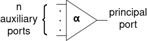
When a cell has n = 0 auxiliary ports, it’s represented as follows:

By connecting a set of cells by wires on their ports we assemble a internet. For instance, a internet with cells α, β and γ, with arities n = 2, 1 and 0, respectively.

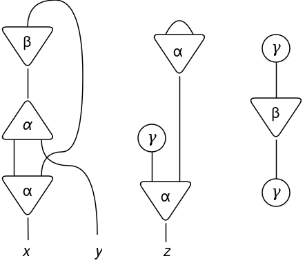
Be aware {that a} wire can join two ports of the identical cell and a internet will not be essentially related. Additionally, on this instance there are three free ports x, y and z.

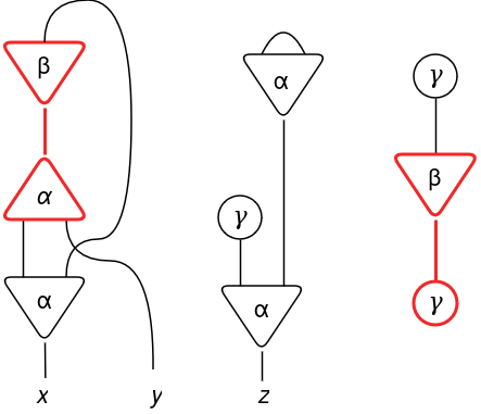
Every time a pair of cells is related by their principal ports, there will probably be an interplay. An interplay is a rule that can modify the internet. This pairs related by their lively ports and able to work together are referred to as an lively pair (or redex).

On the earlier instance, there are two doable interactions (lively pairs) on the primary iteration.

After making use of these guidelines, the internet will probably be modified. We then repeatdly apply these guidelines once more to the ensuing nets till we attain an irreducible type, when no extra interplay guidelines might be utilized. This means of repeatedly making use of interplay guidelines is often known as discount.

An interplay system is constructed with a set of interplay guidelines that may be utilized with out ambiguity. That’s, if we outline an interplay rule for an lively pair (αi, αj), will probably be the identical for all (αi, αj) that seem.

After this transient clarification, let’s do some observe.

Constructing an interplay system for arithmetics

Let’s construct an interplay system for doing arithmetics. To be able to create that, let’s first overlook our primary instinct about numbers and attempt to create a system that may mannequin pure numbers. In 1889, Giuseppe Peano launched 5 axioms to formalize pure numbers, just like how Euclid outlined his axioms for geometry. The Peano’s axioms allow an infinite set to be generated by a finite set of symbols and guidelines. Utilizing these axioms, Peano outlined some guidelines for a finite set of symbols to mannequin pure numbers and their arithmetic properties:

0 → Symbolizes the quantity zero

s(n) → Represents the successor operate. It returns the subsequent pure quantity.

Utilizing s and 0 we are able to outline the pure numbers, as we’ve got beforehand seen throughout lambda calculus research:

1 = s(0)

2 = s(s(0))

3 = s(s(s(0)))

and so on…

+ → Represents addition. It’s a operate recursively outlined as:

Base case: 0 + a = a

Recursion: a + s(b) = s(a+b)

For instance:

a + 3:

= a + s(2)

= s(a+2)

= s(a+s(1))

= s(s(a+1))

= s(s(a+s(0)))

= s(s(s(a+0)))

= s(s(s(a)))

×: Represents multiplication. It’s a operate recursively outlined as:

Base case: b × 0 = 0

Recursion: s(a) × b = (a × b) + b

Impressed by this, Yves Lafont constructed a interplay system to mannequin pure numbers and arithmetics. Let’s perceive:

First, he outlined cells for the s and 0 symbols:

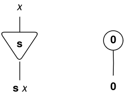
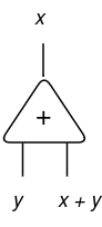
Then, the cell for the addition operation:

It appears unusual, I do know, however I promise will it is going to additional make sense.

If all pure numbers might be expressed utilizing solely the symbols 0 and successor s, for addition we have to outline simply two interplay guidelines: how an addition interacts with successor and with 0. Due to this fact, Lafont launched the 2 following interplay guidelines:

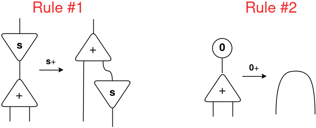
Examine these guidelines with the Peano’s equations for addition, they’re extactly the identical expressions:

s(x) + y = s(x+y)

0 + y = y

Now, let’s perceive the interplay guidelines for multiplication. The cell for multiplication is outlined as follows:

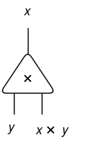
Now, check out Peano’s equations:

y × 0 = 0

s(x) × y = (x × y) + y

Be aware that the primary equation “erases” the y variable (y seems on the left aspect of the equation and don’t seem on the appropriate aspect). Within the second equation, the y is “duplicated” with one other multiplication and an addition.

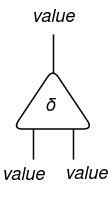
Thus, two different symbols are wanted: ε (eraser) and δ (duplicator).

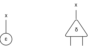
The thought of this symbols is {that a} internet representing pure numbers will probably be erased when related to the principal port of ε, and will probably be duplicated whether it is related to the principal port of δ. Now, the multiplication rule might be represented as follows:

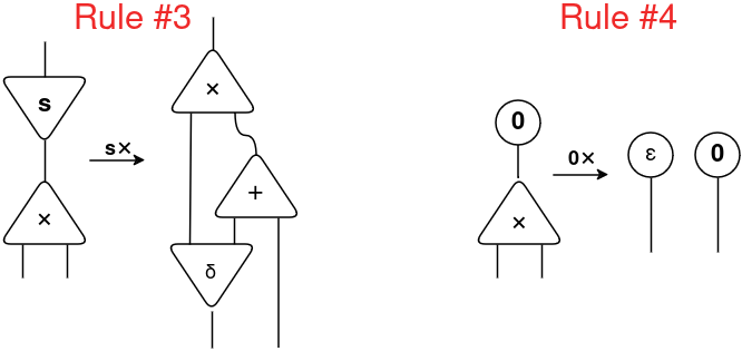
Attempt to replicate on how they’re just like the Peano’s expressions:

s(x) × y = (x × y) + y

y × 0 = 0

The interplay guidelines for duplicator and eraser with successor and 0 are outlined as follows:

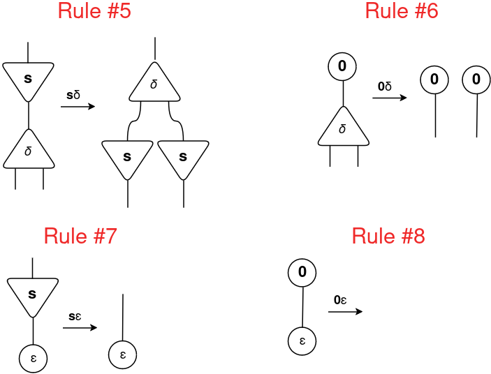
Thus, we’ve got a set of six symbols {0, s, +, ×, δ, ε} with the next set of eight interplay guidelines: {(s, +), (0, +), (s, ×), (0, ×), (s, δ), (0, δ), (s, ε), (0, ε)}. Let’s analyze them in observe for the operation 2 × 2.

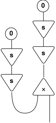
When you have a look, there’s an lively pair (s, ×) that we are able to apply the Rule #3.

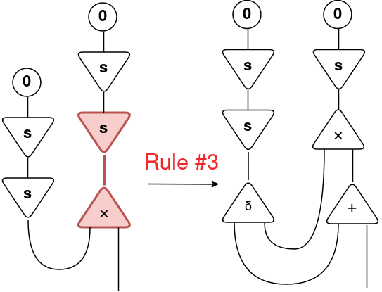
Due to this fact, the operation is solved by making use of the interplay guidelines till we attain an irreducible type:

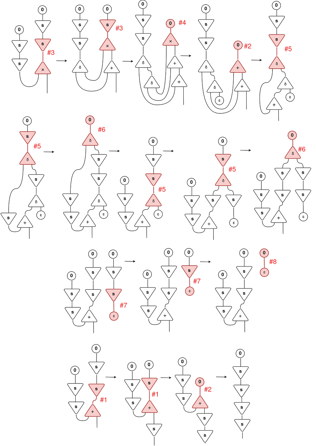
Check out the ultimate type that we’ve got reached: s(s(s(s 0))).

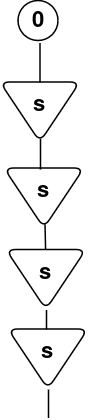
It’s precisely the definition of the numeral 4, the results of 2 × 2! Wonderful, proper? After some manipulation of unusual symbols, we may remedy an arithmetic operation! 😀

However why do such an advanced factor? What are the benefits of fixing issues utilizing these manipulations?

Lafont’s nets have an attention-grabbing property: if a internet μ can cut back in a single step to 2 totally different doable nets v or v’, then v and v’ cut back in a single step to a standard internet ξ.

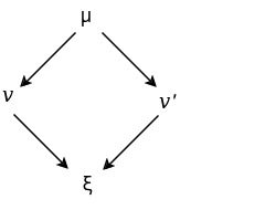
The consequence of this confluence property is that if a internet μ reduces to v in n steps, then any sequence of reductions will attain v in n steps. In different phrases, the order of the applying of interplay guidelines doesn’t matter, the online will attain the identical type with the identical quantity of steps!

Did you get the ability of this property? Mainly, if the order of interactions doesn’t matter, we are able to apply them in parallel! 🤯

As an example, on our earlier 2 × 2 operation, as a substitute of making use of the principles one after the other, we may parallelize them at moments like this:

In precise execution, each guidelines might be parallelized by working them in two separated threads, with out considerations about thread collisions and different widespread points associated to parallelism. And that’s one of many core rules on which HVM/Bend is based! Based mostly on that, all operations that may be parallelized will probably be inherently parallelized!

Now that we perceive interplay nets, let’s take yet one more step. Earlier on this article, I discussed that HVM was primarily based on Interplay Combinators, so let’s perceive how these ideas relate.

Interplay Combinators

Based mostly on his earlier Interplay Nets work, Yves Lafont created the Interplay Combinators. The thought was to create a illustration of computation utilizing a minimal set of primitives, referred to as combinators. Whereas interplay nets use graph rewriting to mannequin computation explicitly, interplay combinators refine this by specializing in the basic combinatory logic. This shift offers a extra summary however extra highly effective framework for expressing computation processes.

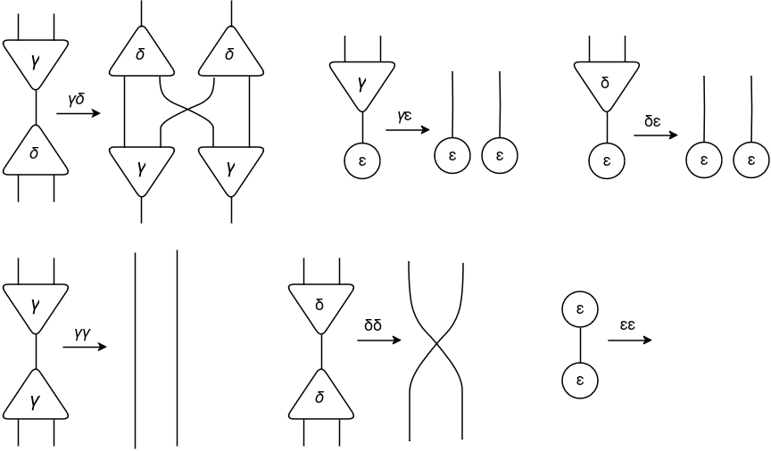
For interplay combinators, Lafont outlined three symbols (additionally referred to as combinators): γ (constructor), δ (duplicator) and ε (eraser).

Utilizing these three combinators, a complete of solely six guidelines have been created. These guidelines are divided into:

commutation — when two cells of various symbols work together (γδ, γε, δε);

annihilation — when two cells of the identical image work together (γγ, δδ, εε).

The principles are outlined beneath:

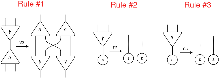
Due to this fact, utilizing solely these six guidelines you may mannequin any computable algorithm! Wonderful, proper?

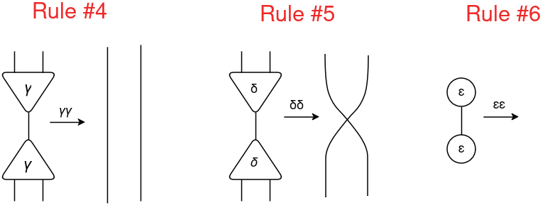
Nonetheless, the HVM runtime makes use of a variant of Lafont’s interplay combinators, referred to as Symmetric Interplay Combinators (SIC) (Mazza, 2007). This variant is a simplified model that makes use of the identical rewrite rule for all of its symbols:

As you may see, the only distinction is that the principles γγ and δδ at the moment are the same. The essential confluence property is maintained, preserving its parallelization functionality.

For now on, we will probably be utilizing the SIC guidelines for our examples, so concentrate on them.

Lambda Calculus → Symmetric Interplay Combinators

Now you could be asking “How can I write applications utilizing that? The right way to remodel my Python operate into interplay combinators drawings?”

I discussed earlier than you could signify any computable algorithm utilizing lambda calculus proper?

Now one other data: you may remodel lambda calculus into interplay combinators!

Thus, any program might be remodeled into lambda calculus, then remodeled into interplay combinators, run in parallel after which be remodeled again!

So, let’s perceive how one can translate lambdas to interplay combinators!

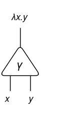
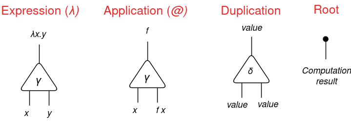
Lambda expressions ( λ ) and purposes ( @ ) might be expressed utilizing a constructor γ. As an example, a lambda expression λx.y might be expressed as follows:

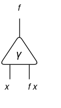
And for a given software f x, we are able to categorical it as follows:

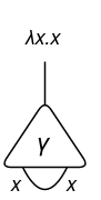
Utilizing these representations, we are able to categorical the id expression λx.x (given x, return x itself):

Now, think about we need to do the software (λx.x)y:

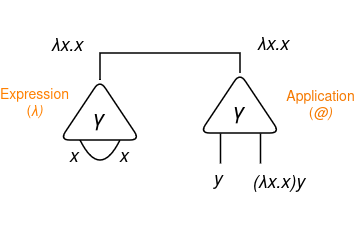
If we cut back the expression (λx.x)y, we’ll get y as consequence. Let’s analyze what can we get utilizing SIC guidelines?

Discover that when there’s an software utilized to a lambda expression, there will probably be an lively pair that we are able to cut back! On this case, we’ll apply the interplay rule γγ. Additionally, for now on, we’ll use a circle to determine the ultimate calculation consequence we’re focused on.

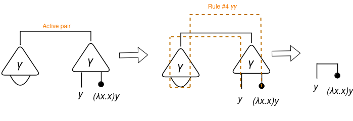
As you may discover, (λx.x)y was appropriately decreased to y! Wonderful, proper?

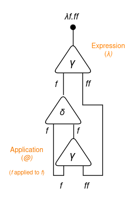
Now, think about we need to categorical λf.ff (given f, apply f to itself). As you may discover, the parameter f is duplicated on the physique. That’s when the duplicator (δ) comes into motion! We will use duplicators to repeat (duplicate) values:

Let’s return to our expression λf.ff. First, determine that that is an expression that given the enter f, it outputs the software f utilized to f itself. Due to this fact, it may be expressed as follows:

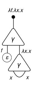
Past duplication, variables may also be vanished. As an example, let’s take the Church quantity 0 := λf.λx.x. This expression might be learn as “given two variables f and x, return x”. As you may discover, the variable f just isn’t used on the output. If we tried to signify utilizing SIC with our present information, we’d get hold of:

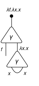
The f wire is floating. One thing appears mistaken, proper? That’s why we’ve got the eraser ε! To be able to signify this variable disappearance we do:

In abstract, we are able to deal with Lambda Calculus with Symmetric Interplay Combinators utilizing:

Examples

Now that we lined these transformations, we’re capable of carry out extra complicated operations.

Church numbers

Let’s draw some Church numbers!

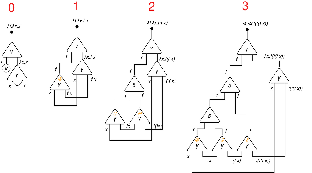
Earlier than we go additional, attempt to replicate this your self! Get a paper and begin drawing! As an example, let’s strive to attract collectively the Church quantity 4: λf.λx.f(f(f(f x))).

The factor that I draw is the outer lambda expression λf.____

Then, the second lambda expression __.λx.____:

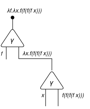
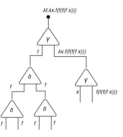
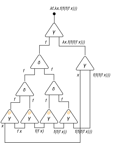
Now, we have to draw the purposes (@). However first, discover that we’ve got f repeated 4 occasions. Due to this fact, we have to copy (duplicate) f three extra occasions (so we want three duplicators in sequence):

Now that we’ve got 4 copies of f, we are able to draw the purposes of f to f in sequence!

Utilizing the identical technique, we are able to simply assemble different expressions.

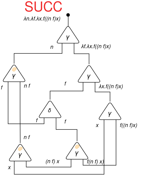
Successor

Let’s implement the successor operate. It’s given by λn.λf.λx.f((n f) x).

Let’s apply SUCC to the quantity 0 and analyze what we get.

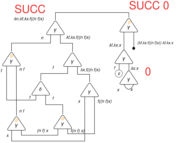
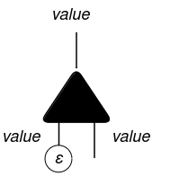
Let’s apply the interplay guidelines. To be able to facilitate readability, I’ll draw duplicators δ as black cells and constructors γ as white cells:

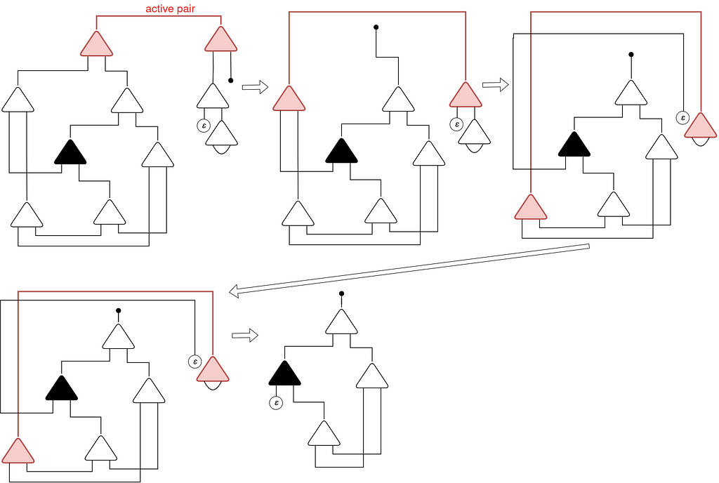
Properly, we must always have reached the Church numeral 1, proper? What went mistaken? Check out the eraser ε related to the auxiliary port of the duplicator δ (in black):

This eraser is making this left auxiliary port to be redundant! All the data handed by this duplicator will probably be erased. For any cell that interacts with this duplicator, the left half will probably be erased.

So we are able to take away this redundant duplicator and join the wire immediately:

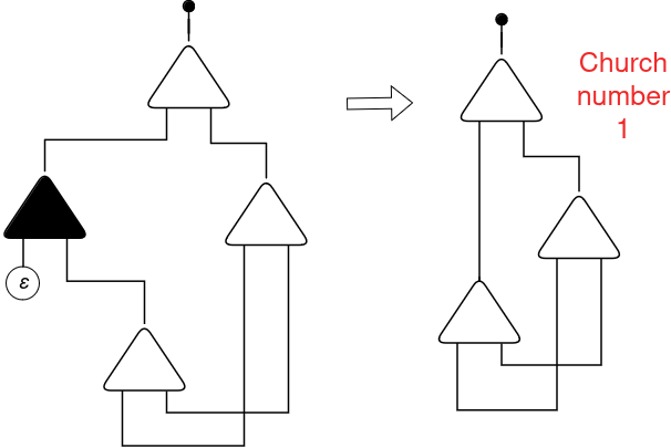
And voila! After decreasing SUCC(0) we acquired precisely the Church no 1, as anticipated!

Let’s apply SUCC againt to the number one and see if we get the quantity 2:

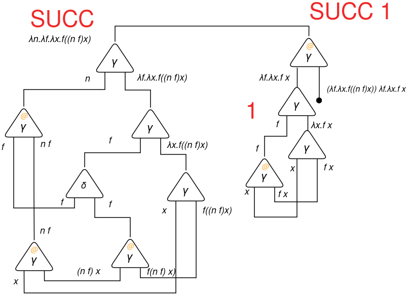
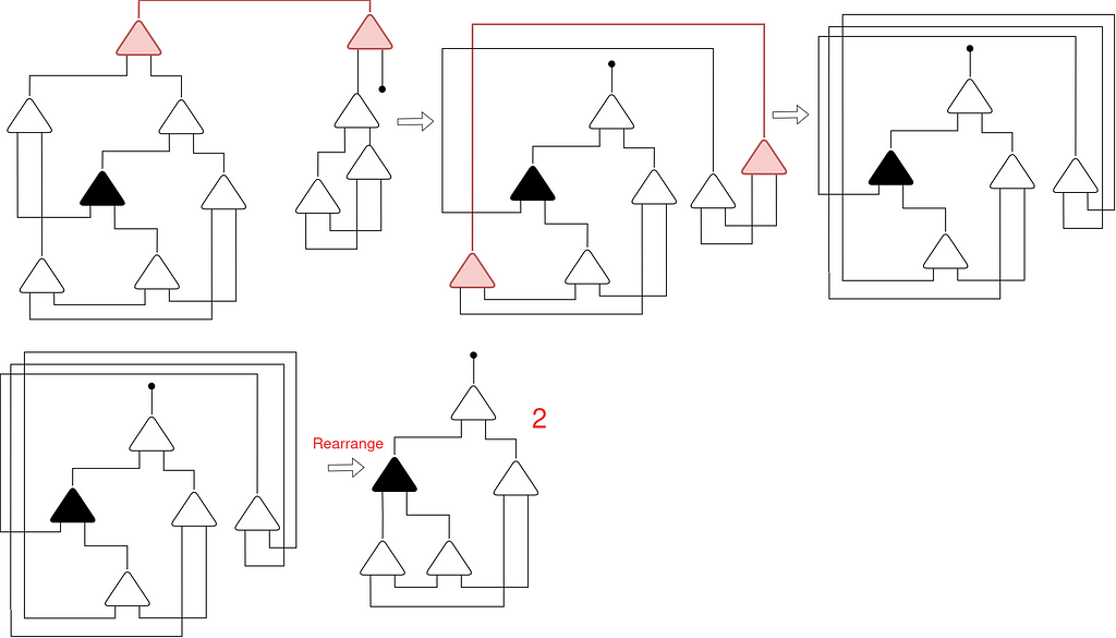
We acquired precisely the Church quantity 2! Wonderful, proper?

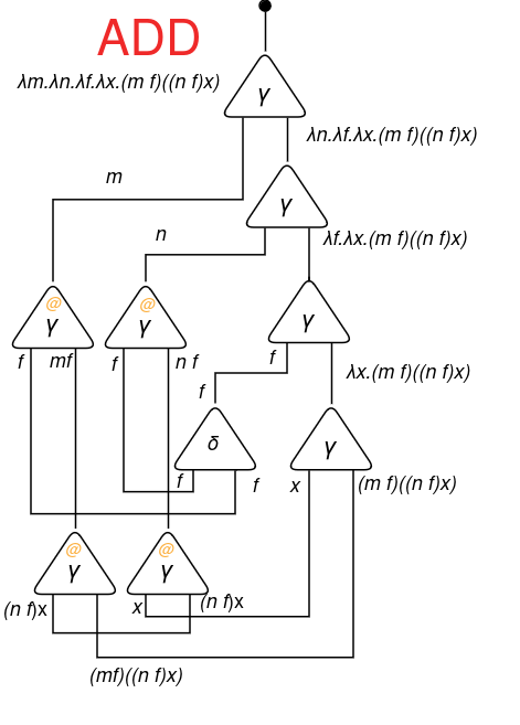
Addition

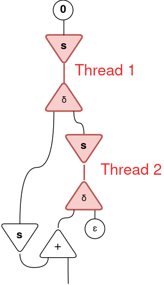
To date, we’ve got simply carried out sequential reductions. Let’s do a extra complicated one, corresponding to addition, to visualise the complete parallelization potential of interplay combinators. Beneath the SIC illustration of addition: ADD(m, n) = λm.λn.λf.λx.(m f)((n f) x).

Let’s calculate ADD 1 1:

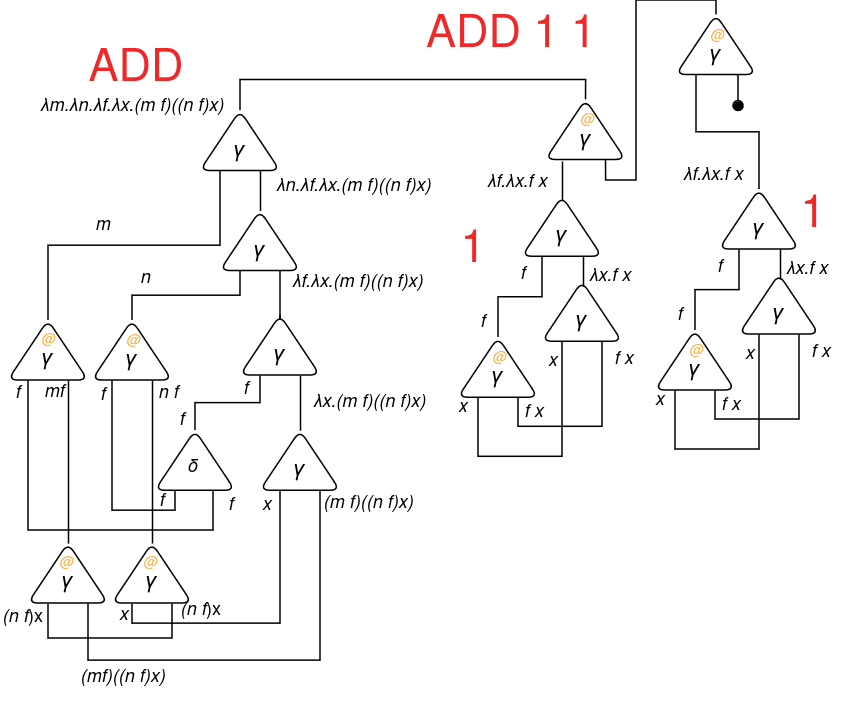
Executing the reductions:

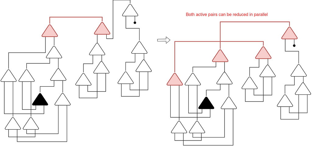
Check out this step. There are two lively pairs! In circumstances like this we are able to cut back each in parallel. In an actual program, we may run them in two totally different threads.

Let’s proceed:

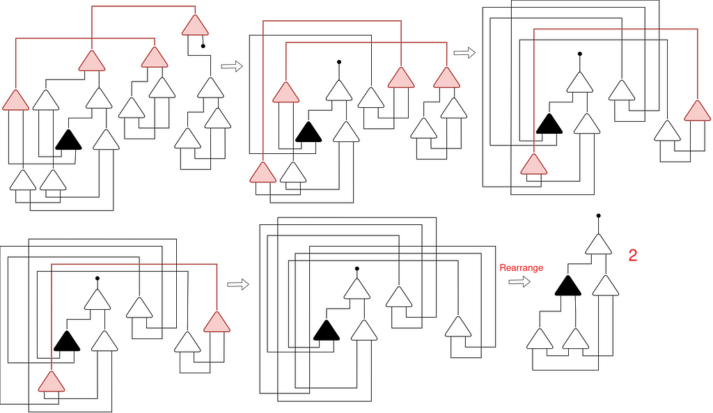
After decreasing ADD 1 1 we acquired precisely the illustration of the Church quantity 2!

And that’s how the operations are parallelized utilizing Interplay Combinators. At every step, if there are multiples lively pairs, all of them run in numerous threads.

Conclusion

On this submit we lined primary ideas of lambda calculus, interplay combinators, and the way they’re mixed to parallelize operations. I hope I may provide you with a quick clarification on how Bend/HVM works and for extra data, please go to their web site.

Additionally, comply with me right here and on my LinkedIn profile to remain up to date on my newest articles!

References

HigherOrderCO web site

Lafont’s Interplay Combinators paper

How HVM works video

Interplay combinators tutorial 1

Interplay combinators tutorial 2

Lambda calculus tutorial

---

How Bend Works: A Parallel Programming Language That “Feels Like Python however Scales Like CUDA” was initially revealed in In direction of Information Science on Medium, the place individuals are persevering with the dialog by highlighting and responding to this story.

Supply hyperlink