


")
 AL15G-52, 39.62cm (15.6 inch) FHD Show, Premium Steel Physique, Metal Grey, 1.99KG")

, RAM (8gb to 16gb), with Trendy Mesh Panel Design On Gaming Cupboard")

 2.8″ Touchscreen Sensible Cell Cellphone Android 11, IP68 Water Resistant, T-Cellular 4G LTE GSM Single Nano Slot")

")

 | Android 13 | Breezy Mint")


Constructing GANs from scratch in python
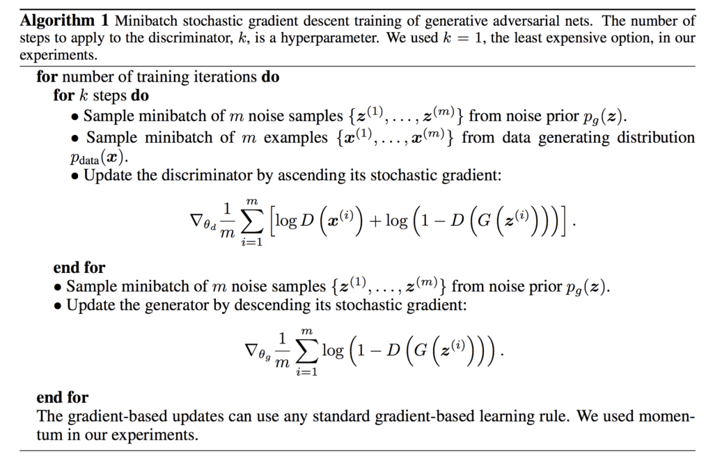
The thought of Generative Adversarial Networks, or GANs, was launched by Goodfellow and his colleagues [1] in 2014, and shortly after that grew to become extraordinarily fashionable within the subject of laptop imaginative and prescient and picture technology. Regardless of the final 10 years of speedy growth throughout the area of AI and progress of the variety of new algorithms, the simplicity and brilliance of this idea are nonetheless extraordinarily spectacular. So at present I need to illustrate how highly effective these networks could be by trying to take away clouds from satellite tv for pc RGB (Crimson, Inexperienced, Blue) photos.
Preparation of a correctly balanced, sufficiently big and appropriately pre-processed CV dataset takes a strong period of time, so I made a decision to discover what Kaggle has to supply. The dataset I discovered probably the most applicable for this process is EuroSat [2], which has an open license. It contains 27000 labeled RGB photos 64×64 pixels from Sentinel-2 and is constructed for fixing the multiclass classification downside.
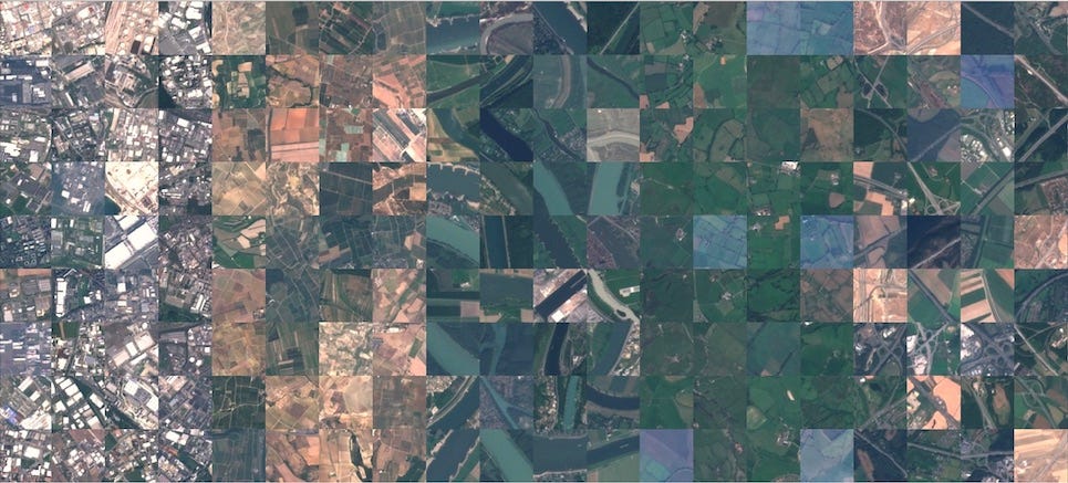
We aren’t concerned with classification itself, however one of many foremost options of the EuroSat dataset is that every one its photos have a transparent sky. That‘s precisely what we want. Adopting this strategy from [3], we’ll use these Sentinel-2 photographs as targets and create inputs by including noise (clouds) to them.
So let’s put together our information earlier than really speaking about GANs. Firstly, we have to obtain the information and merge all of the lessons into one listing.
🐍The total python code: GitHub.
import numpy as np
import pandas as pd
import random

from os import listdir, mkdir, rename
from os.path import be a part of, exists
import shutil
import datetime

import matplotlib.pyplot as plt
from highlight_text import ax_text, fig_text
from PIL import Picture

import warnings

warnings.filterwarnings('ignore')
lessons = listdir('./EuroSat')
path_target = './EuroSat/all_targets'
path_input = './EuroSat/all_inputs'

"""RUN IT ONLY ONCE TO RENAME THE FILES IN THE UNPACKED ARCHIVE"""
mkdir(path_input)
mkdir(path_target)
okay = 1
for form in lessons:
  path = be a part of('./EuroSat', str(form))
  for i, f in enumerate(listdir(path)):
    shutil.copyfile(be a part of(path, f),
                  be a part of(path_target, f))
    rename(be a part of(path_target, f), be a part of(path_target, f'{okay}.jpg'))
    okay += 1
The second essential step is producing noise. Whereas you should utilize totally different approaches, e.g. randomly masking out some pixels, including some Gaussian noise, on this article I need to strive a brand new factor for me — Perlin noise. It was invented within the 80s by Ken Perlin [4] when creating cinematic smoke results. This sort of noise has a extra natural look in comparison with common random noise. Simply let me show it.
def generate_perlin_noise(width, peak, scale, octaves, persistence, lacunarity):
    noise = np.zeros((peak, width))
    for i in vary(peak):
        for j in vary(width):
            noise[i][j] = pnoise2(i / scale,
                                  j / scale,
                                  octaves=octaves,
                                  persistence=persistence,
                                  lacunarity=lacunarity,
                                  repeatx=width,
                                  repeaty=peak,
                                  base=0)
    return noise

def normalize_noise(noise):
    min_val = noise.min()
    max_val = noise.max()
    return (noise - min_val) / (max_val - min_val)

def generate_clouds(width, peak, base_scale, octaves, persistence, lacunarity):
    clouds = np.zeros((peak, width))
    for octave in vary(1, octaves + 1):
        scale = base_scale / octave
        layer = generate_perlin_noise(width, peak, scale, 1, persistence, lacunarity)
        clouds += layer * (persistence ** octave)

    clouds = normalize_noise(clouds)
    return clouds

def overlay_clouds(picture, clouds, alpha=0.5):

    clouds_rgb = np.stack([clouds] * 3, axis=-1)

    picture = picture.astype(float) / 255.0
    clouds_rgb = clouds_rgb.astype(float)

    blended = picture * (1 - alpha) + clouds_rgb * alpha

    blended = (blended * 255).astype(np.uint8)
    return blended
width, peak = 64, 64
octaves = 12 #variety of noise layers mixed
persistence = 0.5 #decrease persistence reduces the amplitude of higher-frequency octaves
lacunarity = 2 #increased lacunarity will increase the frequency of higher-frequency octaves
for i in vary(len(listdir(path_target))):
  base_scale = random.uniform(5,120) #noise frequency
  alpha = random.uniform(0,1) #transparency

  clouds = generate_clouds(width, peak, base_scale, octaves, persistence, lacunarity)

  img = np.asarray(Picture.open(be a part of(path_target, f'{i+1}.jpg')))
  picture = Picture.fromarray(overlay_clouds(img,clouds, alpha))
  picture.save(be a part of(path_input,f'{i+1}.jpg'))
  print(f'Processed {i+1}/{len(listdir(path_target))}')
idx = np.random.randint(27000)
fig,ax = plt.subplots(1,2)
ax[0].imshow(np.asarray(Picture.open(be a part of(path_target, f'{idx}.jpg'))))
ax[1].imshow(np.asarray(Picture.open(be a part of(path_input, f'{idx}.jpg'))))
ax[0].set_title("Goal")
ax[0].axis('off')
ax[1].set_title("Enter")
ax[1].axis('off')
plt.present()
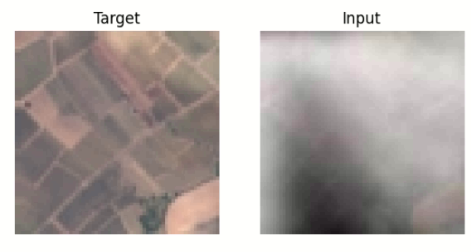
As you’ll be able to see above, the clouds on the pictures are very life like, they’ve totally different “density” and texture resembling the true ones.
If you’re intrigued by Perlin noise as I used to be, here’s a actually cool video on how this noise could be utilized within the GameDev business:
https://medium.com/media/5e59260fbb0a38147329cf292512c9cb/href
Since now we’ve got a ready-to-use dataset, let’s speak about GANs.
Generative Adversarial Community
To raised illustrate this concept, let’s think about that you just’re touring round South-East Asia and end up in an pressing want of a hoodie, because it’s too chilly exterior. Coming to the closest avenue market, you discover a small store with some branded garments. The vendor brings you a pleasant hoodie to strive on saying that it’s the well-known model ExpensiveButNotWorthIt. You are taking a better look and conclude that it’s clearly a pretend. The vendor says: ‘Wait a sec, I’ve the REAL one. He returns with one other hoodie, which appears extra just like the branded one, however nonetheless a pretend. After a number of iterations like this, the vendor brings an indistinguishable copy of the legendary ExpensiveButNotWorthIt and also you readily purchase it. That’s mainly how the GANs work!
Within the case of GANs, you might be referred to as a discriminator (D). The objective of a discriminator is to differentiate between a real object and a pretend one, or to unravel the binary classification process. The vendor is known as a generator (G), since he’s attempting to generate a high-quality pretend. The discriminator and generator are educated independently to outperform one another. Therefore, ultimately we get a high-quality pretend.
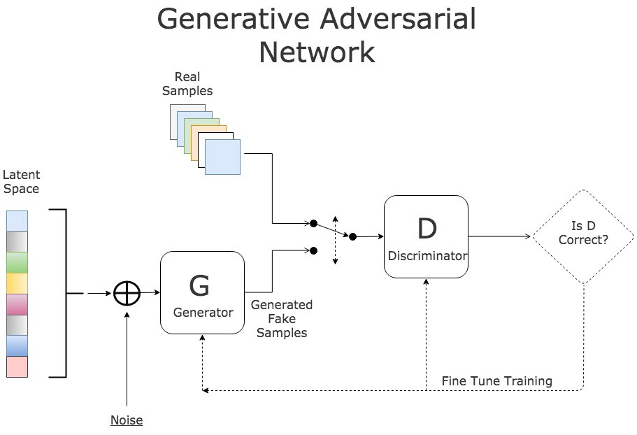
The coaching course of initially appears like this:
- Pattern enter noise (in our case photos with clouds).
- Feed the noise to G and gather the prediction.
- Calculate the D loss by getting 2 predictions one for G’s output and one other for the true information.
- Replace D’s weights.
- Pattern enter noise once more.
- Feed the noise to G and gather the prediction.
- Calculate the G loss by feeding its prediction to D.
- Replace G’s weights.
In different phrases we are able to outline a price operate V(G,D):

the place we need to decrease the time period log(1-D(G(z))) to coach G and maximize log D(x) to coach D (on this notation x — actual information pattern and z — noise).
Now let’s attempt to implement it in pytorch!
Within the authentic paper authors speak about utilizing Multilayer Perceptron (MLP); it’s additionally typically referred merely as ANN, however I need to strive somewhat bit extra sophisticated strategy — I need to use the UNet [5] structure as a Generator and ResNet [6] as a Discriminator. These are each well-known CNN architectures, so I gained’t be explaining them right here (let me know if I ought to write a separate article within the feedback).
Let’s construct them. Discriminator:
import torch
import torch.nn as nn
import torch.optim as optim
import torch.nn.purposeful as F
from torch.utils.information import Dataset, DataLoader
from torchvision import transforms
from torch.utils.information import Subset
class ResidualBlock(nn.Module):
    def __init__(self, in_channels, out_channels, stride = 1, downsample = None):
        tremendous(ResidualBlock, self).__init__()
        self.conv1 = nn.Sequential(
                        nn.Conv2d(in_channels, out_channels, kernel_size = 3, stride = stride, padding = 1),
                        nn.BatchNorm2d(out_channels),
                        nn.ReLU())
        self.conv2 = nn.Sequential(
                        nn.Conv2d(out_channels, out_channels, kernel_size = 3, stride = 1, padding = 1),
                        nn.BatchNorm2d(out_channels))
        self.downsample = downsample
        self.relu = nn.ReLU()
        self.out_channels = out_channels

    def ahead(self, x):
        residual = x
        out = self.conv1(x)
        out = self.conv2(out)
        if self.downsample:
            residual = self.downsample(x)
        out += residual
        out = self.relu(out)
        return out


class ResNet(nn.Module):
    def __init__(self, block=ResidualBlock, all_connections=[3,4,6,3]):
        tremendous(ResNet, self).__init__()
        self.inputs = 16
        self.conv1 = nn.Sequential(
                        nn.Conv2d(3, 16, kernel_size = 3, stride = 1, padding = 1),
                        nn.BatchNorm2d(16),
                        nn.ReLU()) #16x64x64
        self.maxpool = nn.MaxPool2d(kernel_size = 2, stride = 2) #16x32x32


        self.layer0 = self.makeLayer(block, 16, all_connections[0], stride = 1) #connections = 3, form: 16x32x32
        self.layer1 = self.makeLayer(block, 32, all_connections[1], stride = 2)#connections = 4, form: 32x16x16
        self.layer2 = self.makeLayer(block, 128, all_connections[2], stride = 2)#connections = 6, form: 1281x8x8
        self.layer3 = self.makeLayer(block, 256, all_connections[3], stride = 2)#connections = 3, form: 256x4x4
        self.avgpool = nn.AvgPool2d(4, stride=1)
        self.fc = nn.Linear(256, 1)

    def makeLayer(self, block, outputs, connections, stride=1):
        downsample = None
        if stride != 1 or self.inputs != outputs:
            downsample = nn.Sequential(
                nn.Conv2d(self.inputs, outputs, kernel_size=1, stride=stride),
                nn.BatchNorm2d(outputs),
            )
        layers = []
        layers.append(block(self.inputs, outputs, stride, downsample))
        self.inputs = outputs
        for i in vary(1, connections):
            layers.append(block(self.inputs, outputs))

        return nn.Sequential(*layers)


    def ahead(self, x):
        x = self.conv1(x)
        x = self.maxpool(x)
        x = self.layer0(x)
        x = self.layer1(x)
        x = self.layer2(x)
        x = self.layer3(x)
        x = self.avgpool(x)
        x = x.view(-1, 256)
        x = self.fc(x).flatten()
        return F.sigmoid(x)
Generator:
class DoubleConv(nn.Module):
    def __init__(self, in_channels, out_channels):
        tremendous(DoubleConv, self).__init__()
        self.double_conv = nn.Sequential(
            nn.Conv2d(in_channels, out_channels, kernel_size=3, padding=1),
            nn.BatchNorm2d(out_channels),
            nn.ReLU(inplace=True),
            nn.Conv2d(out_channels, out_channels, kernel_size=3, padding=1),
            nn.BatchNorm2d(out_channels),
            nn.ReLU(inplace=True)
        )

    def ahead(self, x):
        return self.double_conv(x)

class UNet(nn.Module):
    def __init__(self):
      tremendous().__init__()
      self.conv_1 = DoubleConv(3, 32) # 32x64x64
      self.pool_1 = nn.MaxPool2d(kernel_size=2, stride=2) # 32x32x32

      self.conv_2 = DoubleConv(32, 64)  #64x32x32
      self.pool_2 = nn.MaxPool2d(kernel_size=2, stride=2) #64x16x16

      self.conv_3 = DoubleConv(64, 128)  #128x16x16
      self.pool_3 = nn.MaxPool2d(kernel_size=2, stride=2) #128x8x8

      self.conv_4 = DoubleConv(128, 256)  #256x8x8
      self.pool_4 = nn.MaxPool2d(kernel_size=2, stride=2) #256x4x4

      self.conv_5 = DoubleConv(256, 512)  #512x2x2

      #DECODER
      self.upconv_1 = nn.ConvTranspose2d(512, 256, kernel_size=2, stride=2) #256x4x4
      self.conv_6 = DoubleConv(512, 256) #256x4x4


      self.upconv_2 = nn.ConvTranspose2d(256, 128, kernel_size=2, stride=2) #128x8x8
      self.conv_7 = DoubleConv(256, 128)  #128x8x8

      self.upconv_3 = nn.ConvTranspose2d(128, 64, kernel_size=2, stride=2) #64x16x16
      self.conv_8 = DoubleConv(128, 64)  #64x16x16

      self.upconv_4 = nn.ConvTranspose2d(64, 32, kernel_size=2, stride=2) #32x32x32
      self.conv_9 = DoubleConv(64, 32)  #32x32x32

      self.output = nn.Conv2d(32, 3, kernel_size = 3, stride = 1, padding = 1) #3x64x64

    def ahead(self, batch):

      conv_1_out = self.conv_1(batch)
      conv_2_out = self.conv_2(self.pool_1(conv_1_out))
      conv_3_out = self.conv_3(self.pool_2(conv_2_out))
      conv_4_out = self.conv_4(self.pool_3(conv_3_out))
      conv_5_out = self.conv_5(self.pool_4(conv_4_out))

      conv_6_out = self.conv_6(torch.cat([self.upconv_1(conv_5_out), conv_4_out], dim=1))
      conv_7_out = self.conv_7(torch.cat([self.upconv_2(conv_6_out), conv_3_out], dim=1))
      conv_8_out = self.conv_8(torch.cat([self.upconv_3(conv_7_out), conv_2_out], dim=1))
      conv_9_out = self.conv_9(torch.cat([self.upconv_4(conv_8_out), conv_1_out], dim=1))

      output = self.output(conv_9_out)


      return F.sigmoid(output)
Now we have to cut up our information into practice/take a look at and wrap them right into a torch dataset:
class dataset(Dataset):
  def __init__(self, batch_size, images_paths, targets, img_size = 64):
    self.batch_size = batch_size
    self.img_size = img_size
    self.images_paths = images_paths
    self.targets = targets
    self.len = len(self.images_paths) // batch_size

    self.rework = transforms.Compose([
                transforms.ToTensor(),
                ])


    self.batch_im = [self.images_paths[idx * self.batch_size:(idx + 1) * self.batch_size] for idx in vary(self.len)]
    self.batch_t = [self.targets[idx * self.batch_size:(idx + 1) * self.batch_size] for idx in vary(self.len)]

  def __getitem__(self, idx):
      pred = torch.stack([
              self.transform(Image.open(join(path_input,file_name)))
              for file_name in self.batch_im[idx]
          ])
      goal = torch.stack([
              self.transform(Image.open(join(path_target,file_name)))
              for file_name in self.batch_im[idx]
          ])
      return pred, goal

  def __len__(self):
      return self.len
Good. It’s time to write down the coaching loop. Earlier than doing so, let’s outline our loss capabilities and optimizer:
system = torch.system("cuda" if torch.cuda.is_available() else "cpu")

batch_size = 64
num_epochs = 15
learning_rate_D = 1e-5
learning_rate_G = 1e-4

discriminator = ResNet()
generator = UNet()

bce = nn.BCEWithLogitsLoss()
l1loss = nn.L1Loss()

optimizer_D = optim.Adam(discriminator.parameters(), lr=learning_rate_D)
optimizer_G = optim.Adam(generator.parameters(), lr=learning_rate_G)

scheduler_D = optim.lr_scheduler.StepLR(optimizer_D, step_size=10, gamma=0.1)
scheduler_G = optim.lr_scheduler.StepLR(optimizer_G, step_size=10, gamma=0.1)
As you’ll be able to see, these losses are totally different from the image with the GAN algorithm. Specifically, I added L1Loss. The thought is that we’re not merely producing a random picture from noise, we need to preserve a lot of the info from the enter and simply take away noise. So G loss will be:
G_loss = log(1 − D(G(z))) + 𝝀 |G(z)-y|
as a substitute of simply
G_loss = log(1 − D(G(z)))
𝝀 is an arbitrary coefficient, which balances two elements of the losses.
Lastly, let’s cut up the information to begin the coaching course of:
test_ratio, train_ratio = 0.3, 0.7
num_test = int(len(listdir(path_target))*test_ratio)
num_train = int((int(len(listdir(path_target)))-num_test))

img_size = (64, 64)

print("Variety of practice samples:", num_train)
print("Variety of take a look at samples:", num_test)

random.seed(231)
train_idxs = np.array(random.pattern(vary(num_test+num_train), num_train))
masks = np.ones(num_train+num_test, dtype=bool)
masks[train_idxs] = False

photos = {}
options = random.pattern(listdir(path_input),num_test+num_train)
targets = random.pattern(listdir(path_target),num_test+num_train)

random.Random(231).shuffle(options)
random.Random(231).shuffle(targets)

train_input_img_paths = np.array(options)[train_idxs]
train_target_img_path = np.array(targets)[train_idxs]
test_input_img_paths = np.array(options)[mask]
test_target_img_path = np.array(targets)[mask]

train_loader = dataset(batch_size=batch_size, img_size=img_size, images_paths=train_input_img_paths, targets=train_target_img_path)
test_loader = dataset(batch_size=batch_size, img_size=img_size, images_paths=test_input_img_paths, targets=test_target_img_path)
Now we are able to run our coaching loop:
train_loss_G, train_loss_D, val_loss_G, val_loss_D = [], [], [], []
all_loss_G, all_loss_D = [], []
best_generator_epoch_val_loss, best_discriminator_epoch_val_loss = -np.inf, -np.inf
for epoch in vary(num_epochs):

    discriminator.practice()
    generator.practice()

    discriminator_epoch_loss, generator_epoch_loss = 0, 0

    for inputs, targets in train_loader:
        inputs, true = inputs, targets

        '''1. Coaching the Discriminator (ResNet)'''
        optimizer_D.zero_grad()

        pretend = generator(inputs).detach()

        pred_fake = discriminator(pretend).to(system)
        loss_fake = bce(pred_fake, torch.zeros(batch_size, system=system))

        pred_real = discriminator(true).to(system)
        loss_real = bce(pred_real, torch.ones(batch_size, system=system))

        loss_D = (loss_fake+loss_real)/2

        loss_D.backward()
        optimizer_D.step()

        discriminator_epoch_loss += loss_D.merchandise()
        all_loss_D.append(loss_D.merchandise())

        '''2. Coaching the Generator (UNet)'''
        optimizer_G.zero_grad()

        pretend = generator(inputs)
        pred_fake = discriminator(pretend).to(system)

        loss_G_bce = bce(pred_fake, torch.ones_like(pred_fake, system=system))
        loss_G_l1 = l1loss(pretend, targets)*100
        loss_G = loss_G_bce + loss_G_l1
        loss_G.backward()
        optimizer_G.step()

        generator_epoch_loss += loss_G.merchandise()
        all_loss_G.append(loss_G.merchandise())

    discriminator_epoch_loss /= len(train_loader)
    generator_epoch_loss /= len(train_loader)
    train_loss_D.append(discriminator_epoch_loss)
    train_loss_G.append(generator_epoch_loss)

    discriminator.eval()
    generator.eval()

    discriminator_epoch_val_loss, generator_epoch_val_loss = 0, 0

    with torch.no_grad():
        for inputs, targets in test_loader:
            inputs, targets = inputs, targets

            pretend = generator(inputs)
            pred = discriminator(pretend).to(system)

            loss_G_bce = bce(pretend, torch.ones_like(pretend, system=system))
            loss_G_l1 = l1loss(pretend, targets)*100
            loss_G = loss_G_bce + loss_G_l1
            loss_D = bce(pred.to(system), torch.zeros(batch_size, system=system))

            discriminator_epoch_val_loss += loss_D.merchandise()
            generator_epoch_val_loss += loss_G.merchandise()

    discriminator_epoch_val_loss /= len(test_loader)
    generator_epoch_val_loss /= len(test_loader)

    val_loss_D.append(discriminator_epoch_val_loss)
    val_loss_G.append(generator_epoch_val_loss)

    print(f"------Epoch [{epoch+1}/{num_epochs}]------nTrain Loss D: {discriminator_epoch_loss:.4f}, Val Loss D: {discriminator_epoch_val_loss:.4f}")
    print(f'Prepare Loss G: {generator_epoch_loss:.4f}, Val Loss G: {generator_epoch_val_loss:.4f}')

    if discriminator_epoch_val_loss > best_discriminator_epoch_val_loss:
        discriminator_epoch_val_loss = best_discriminator_epoch_val_loss
        torch.save(discriminator.state_dict(), "discriminator.pth")
    if generator_epoch_val_loss > best_generator_epoch_val_loss:
        generator_epoch_val_loss = best_generator_epoch_val_loss
        torch.save(generator.state_dict(), "generator.pth")
    #scheduler_D.step()
    #scheduler_G.step()

    fig, ax = plt.subplots(1,3)
    ax[0].imshow(np.transpose(inputs.numpy()[7], (1,2,0)))
    ax[1].imshow(np.transpose(targets.numpy()[7], (1,2,0)))
    ax[2].imshow(np.transpose(pretend.detach().numpy()[7], (1,2,0)))
    plt.present()
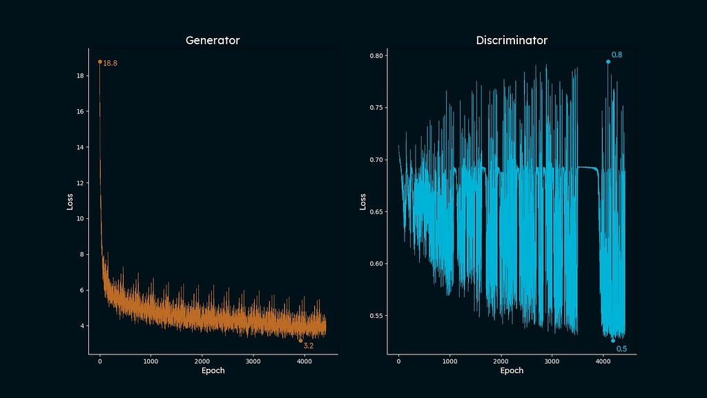
After the code is completed we are able to plot the losses. This code was partly adopted from this cool web site:
from matplotlib.font_manager import FontProperties

background_color = '#001219'
font = FontProperties(fname='LexendDeca-VariableFont_wght.ttf')
fig, ax = plt.subplots(1, 2, figsize=(16, 9))
fig.set_facecolor(background_color)
ax[0].set_facecolor(background_color)
ax[1].set_facecolor(background_color)

ax[0].plot(vary(len(all_loss_G)), all_loss_G, shade='#bc6c25', lw=0.5)
ax[1].plot(vary(len(all_loss_D)), all_loss_D, shade='#00b4d8', lw=0.5)

ax[0].scatter(
      [np.array(all_loss_G).argmax(), np.array(all_loss_G).argmin()],
      [np.array(all_loss_G).max(), np.array(all_loss_G).min()],
      s=30, shade='#bc6c25',
   )
ax[1].scatter(
      [np.array(all_loss_D).argmax(), np.array(all_loss_D).argmin()],
      [np.array(all_loss_D).max(), np.array(all_loss_D).min()],
      s=30, shade='#00b4d8',
   )

ax_text(
      np.array(all_loss_G).argmax()+60, np.array(all_loss_G).max()+0.1,
      f'{spherical(np.array(all_loss_G).max(),1)}',
      fontsize=13, shade='#bc6c25',
      font=font,
      ax=ax[0]
   )
ax_text(
      np.array(all_loss_G).argmin()+60, np.array(all_loss_G).min()-0.1,
      f'{spherical(np.array(all_loss_G).min(),1)}',
      fontsize=13, shade='#bc6c25',
      font=font,
      ax=ax[0]
   )

ax_text(
      np.array(all_loss_D).argmax()+60, np.array(all_loss_D).max()+0.01,
      f'{spherical(np.array(all_loss_D).max(),1)}',
      fontsize=13, shade='#00b4d8',
      font=font,
      ax=ax[1]
   )
ax_text(
      np.array(all_loss_D).argmin()+60, np.array(all_loss_D).min()-0.005,
      f'{spherical(np.array(all_loss_D).min(),1)}',
      fontsize=13, shade='#00b4d8',
      font=font,
      ax=ax[1]
   )
for i in vary(2):
    ax[i].tick_params(axis='x', colours='white')
    ax[i].tick_params(axis='y', colours='white')
    ax[i].spines['left'].set_color('white')
    ax[i].spines['bottom'].set_color('white')
    ax[i].set_xlabel('Epoch', shade='white', fontproperties=font, fontsize=13)
    ax[i].set_ylabel('Loss', shade='white', fontproperties=font, fontsize=13)

ax[0].set_title('Generator', shade='white', fontproperties=font, fontsize=18)
ax[1].set_title('Discriminator', shade='white', fontproperties=font, fontsize=18)
plt.savefig('Loss.jpg')
plt.present()
# ax[0].set_axis_off()
# ax[1].set_axis_off()
And in addition visualize a random pattern from the take a look at dataset:
random.Random(2).shuffle(test_target_img_path)
random.Random(2).shuffle(test_input_img_paths)
subset_loader = dataset(batch_size=5, img_size=img_size, images_paths=test_input_img_paths,
                        targets=test_target_img_path)
generator = UNet()
generator.load_state_dict(torch.load('generator.pth'))

generator.eval()
for X, y in subset_loader:
    fig, axes = plt.subplots(5, 3, figsize=(9, 9))

    for i in vary(5):
        axes[i, 0].imshow(np.transpose(X.numpy()[i], (1, 2, 0)))
        axes[i, 0].set_title("Enter")
        axes[i, 0].axis('off')

        axes[i, 1].imshow(np.transpose(y.numpy()[i], (1, 2, 0)))
        axes[i, 1].set_title("Goal")
        axes[i, 1].axis('off')

        generated_image = generator(X[i].unsqueeze(0)).detach().numpy()[0]
        axes[i, 2].imshow(np.transpose(generated_image, (1, 2, 0)))
        axes[i, 2].set_title("Generated")
        axes[i, 2].axis('off')

    # Modify structure
    plt.tight_layout()
    plt.savefig('Take a look at.jpg')
    plt.present()
    break
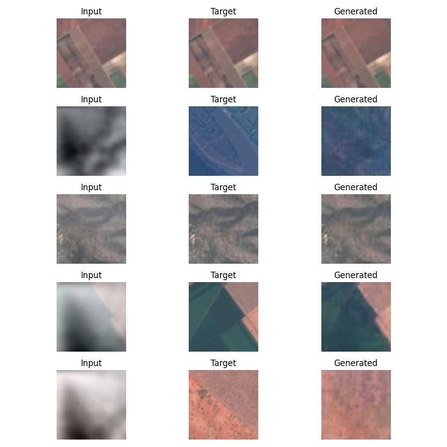
As you’ll be able to see, the outcomes are usually not excellent and rely loads on the land cowl sort. Nonetheless, the constructed mannequin actually removes the clouds from photos and its efficiency could be improved by rising G and D depth. One other promising technique to check is coaching separate fashions for various land cowl varieties. As an illustration, crop fields and water basins are undoubtedly have fairly distinct spatial options, so it’d impact mannequin’s capability to generalize.
I hope this text supplied you with a recent perspective on making use of Deep Studying algorithms within the geospatial area. In my view, GANs are among the many strongest instruments an information scientist can make the most of, and I hope they turn into an important a part of your toolkit as properly!
===========================================
References:
1. Goodfellow, Ian, Jean Pouget-Abadie, Mehdi Mirza, Bing Xu, David Warde-Farley, Sherjil Ozair, Aaron Courville, and Yoshua Bengio. “Generative adversarial nets.” Advances in neural info processing techniques 27 (2014). https://proceedings.neurips.cc/paper_files/paper/2014/file/5ca3e9b122f61f8f06494c97b1afccf3-Paper.pdf
2. Helber, Patrick, Benjamin Bischke, Andreas Dengel, and Damian Borth. “Eurosat: A novel dataset and deep studying benchmark for land use and land cowl classification.” IEEE Journal of Chosen Matters in Utilized Earth Observations and Distant Sensing 12, no. 7 (2019): 2217–2226. https://arxiv.org/pdf/1709.00029
3. Wen, Xue, Zongxu Pan, Yuxin Hu, and Jiayin Liu. “Generative adversarial studying in YUV shade house for skinny cloud elimination on satellite tv for pc imagery.” Distant Sensing 13, no. 6 (2021): 1079. https://www.mdpi.com/2072-4292/13/6/1079
4. Perlin, Ken. “A picture synthesizer.” ACM Siggraph Pc Graphics 19, no. 3 (1985): 287–296. https://dl.acm.org/doi/pdf/10.1145/325165.325247
5. Ronneberger, Olaf, Philipp Fischer, and Thomas Brox. “U-net: Convolutional networks for biomedical picture segmentation.” In Medical picture computing and computer-assisted intervention–MICCAI 2015: 18th worldwide convention, Munich, Germany, October 5–9, 2015, proceedings, half III 18, pp. 234–241. Springer Worldwide Publishing, 2015. https://arxiv.org/pdf/1505.04597
6. He, Kaiming, et al. “Deep residual studying for picture recognition.” Proceedings of the IEEE convention on laptop imaginative and prescient and sample recognition. 2016.https://openaccess.thecvf.com/content_cvpr_2016/papers/He_Deep_Residual_Learning_CVPR_2016_paper.pdf
===========================================
All my publications on Medium are free and open-access, that’s why I’d actually admire in case you adopted me right here!
P.s. I’m extraordinarily keen about (Geo)Knowledge Science, ML/AI and Local weather Change. So if you wish to work collectively on some challenge pls contact me in LinkedIn.
🛰️Comply with for extra🛰️
Erasing Clouds from Satellite tv for pc Imagery Utilizing GANs (Generative Adversarial Networks) was initially printed in In direction of Knowledge Science on Medium, the place persons are persevering with the dialog by highlighting and responding to this story.